
Fig. 1.
Fig. 2.
Fig. 3.
Fig. 4.
Fig. 5.
Fig. 6.
Fig. 7.
Fig. 8.
Fig. 9.
Fig. 10.
Fig. 11.
Fig. 12.
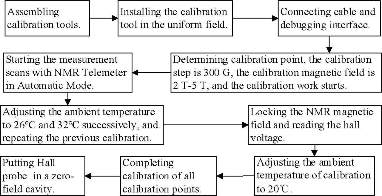
Fig. 13.
Fig. 14.
Fig. 15.
Fig. 16.
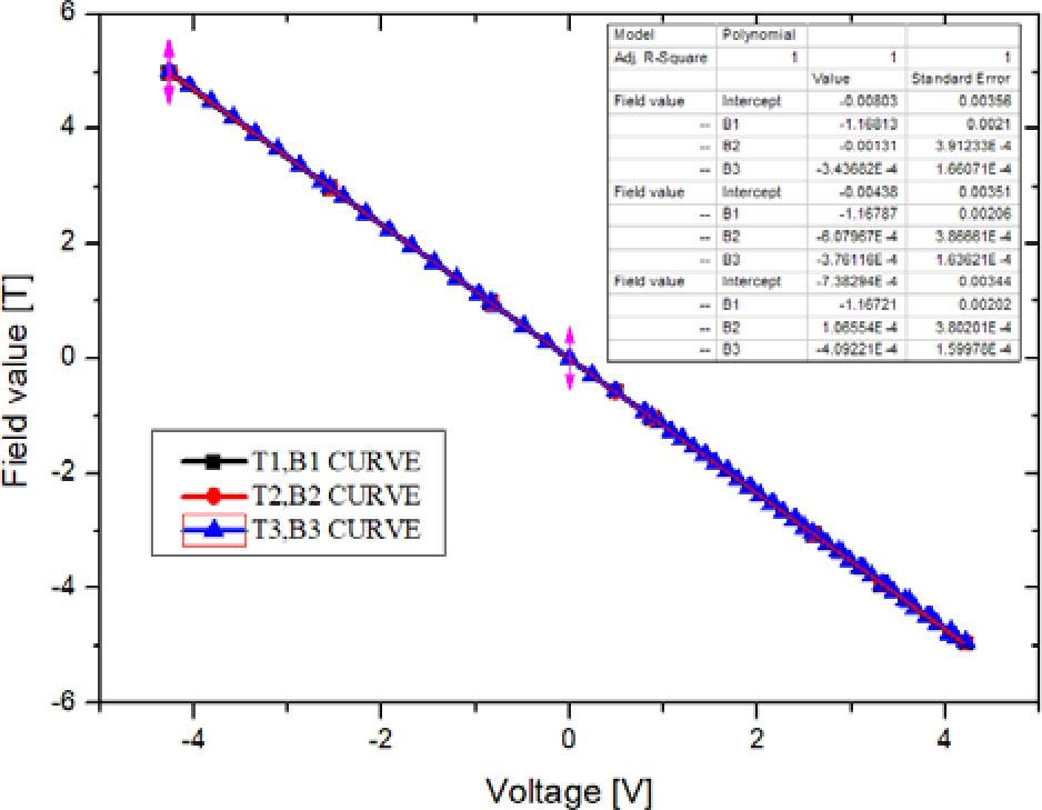
Fig. 17.
Fig. 18.
Fitting results of polynomial Bpol1
| Temperature, T | Polynomial fitting Bpol1 formula |
|---|---|
| T1 = 20°C | Bpol1 = −0.0080 − 1.1681*U − 0.0013*U2 − 3.4368e-4*U3 |
| T2 = 26°C | Bpol1 = −0.0044 − 1.1681*U − 6.080e-4*U2 − 3.7612e-4*U3 |
| T3 = 32°C | Bpol1 = −7.3829e-4 − 1.1672*U + 1.066e-4*U2 − 4.0922e-4*U3 |
Accuracy requirements of calibration
| Requirements | Numerical value |
|---|---|
| Calibration range (T) | 2–5 |
| Calibration step (Gs) | 300 |
| Accuracy | <(0.001% × reading + 0.005% × range) |
| Resolution (Gs) | 0.2–0.4 |