Fig. 1.
Fig. 2.
Fig. 3.
Fig. 4.
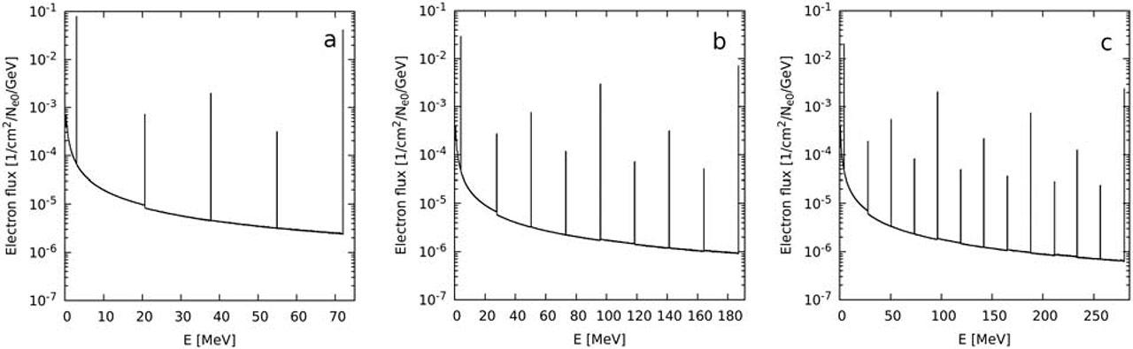
Fig. 5.
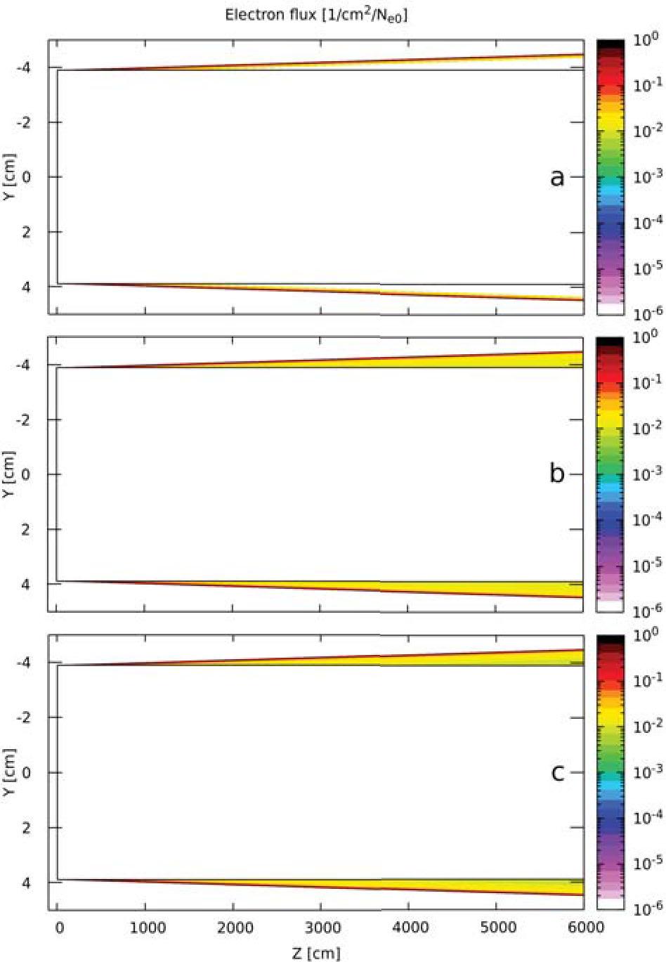
Fig. 6.
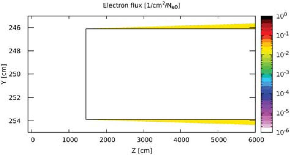
Fig. 7.
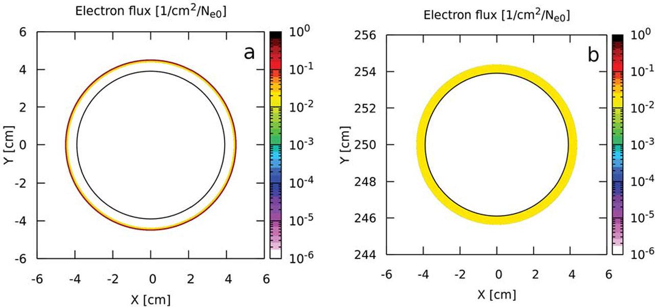
Fig. 8.
Summary of calculated electron fluxes lost from a cylinder with a radius of 3_9 cm to provide a beam loss of 1 W/m_ This radius corresponds to the radius of the designed beam pipe
| Electron energy (MeV) | Φnoacc (e/s) | Φacc (e/s) | Φ (e/s) |
|---|---|---|---|
| 72 | 1.5840 × 10¹³ | 2.152 × 10¹² | 1.7991 × 10¹³ |
| 187 | 9.729 × 10¹² | 1.808 × 10¹² | 1.1537 × 10¹³ |
| 280 | 9.097 × 10¹² | 1.915 × 10¹² | 1.1012 × 10¹³ |