
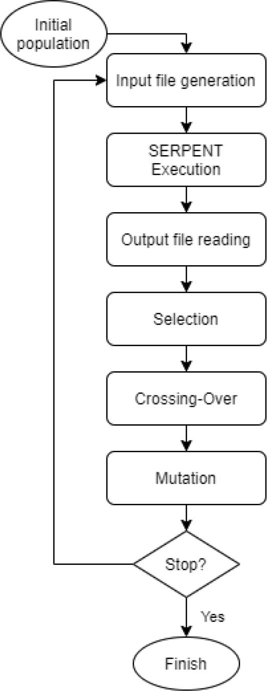
Fig. 1
General algorithm of the computational framework.
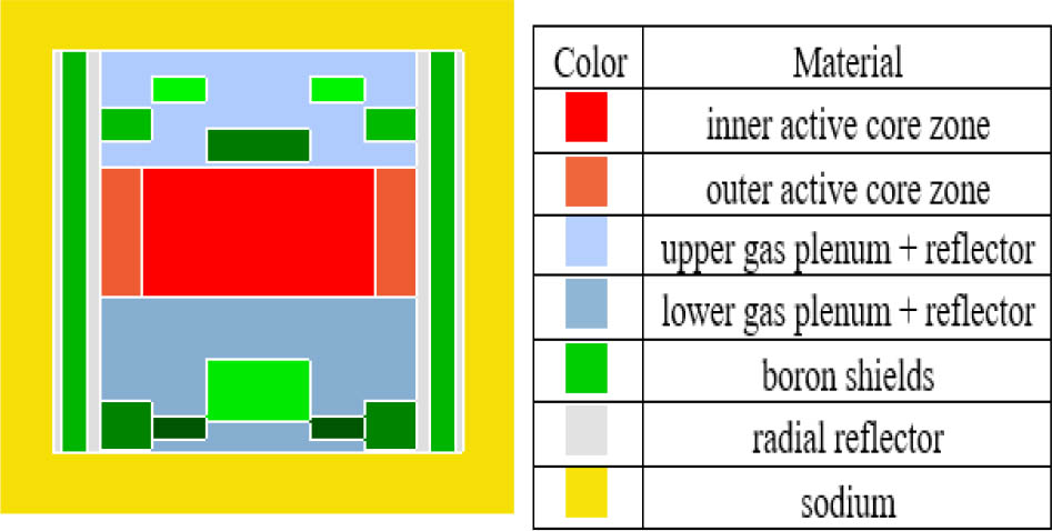
Fig. 2
Axial layout of a sample model with boron shields.
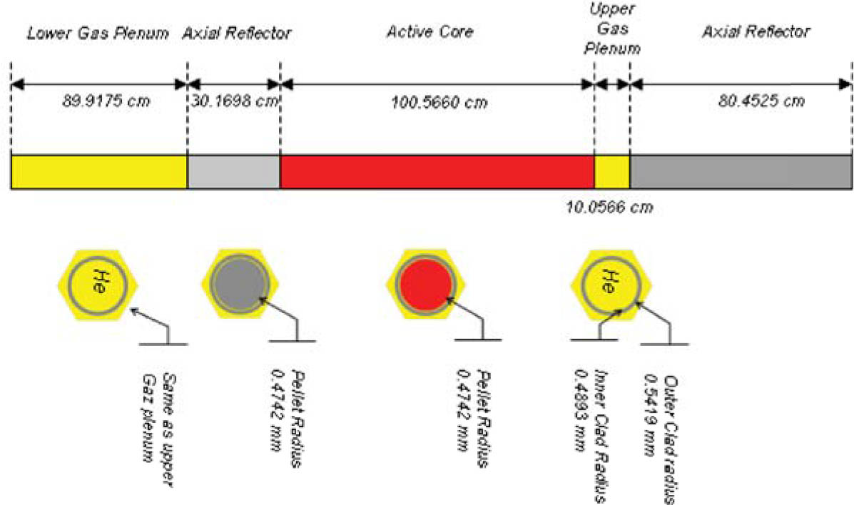
Fig. 3
Axial layout of a single fuel rod with cross sections. Taken from [1].
Table 1
Selected parameters of the best individual from each generation
| Generation | Max(fi) * 106 | knormal | Kvoid | SVR (pcm) | Error (SVR) (pcm) | |
|---|---|---|---|---|---|---|
| 1 | 609.6 | 50.2 | 1.00376 | 1.02770 | 2422 | 12 |
| 2 | 681.7 | 60.6 | 0.99744 | 1.02136 | 2348 | 12 |
| 3 | 692.7 | 66.4 | 0.99703 | 1.02059 | 2316 | 12 |
| 4 | 782.0 | 70.1 | 0.99526 | 1.01849 | 2292 | 12 |
| 5 | 795.4 | 67.1 | 0.99798 | 1.02157 | 2314 | 12 |
| 6 | 989.3 | 65.9 | 0.99654 | 1.02009 | 2317 | 12 |
| 7 | 1048.3 | 66.8 | 0.99709 | 1.02063 | 2314 | 12 |
| 8 | 1059.2 | 74.3 | 0.99548 | 1.01850 | 2270 | 12 |
| 9 | 1088.5 | 93.7 | 0.99222 | 1.01402 | 2167 | 12 |
| 10 | 1177.2 | 95.1 | 0.99391 | 1.01576 | 2164 | 12 |
| 11 | 1331.2 | 101.3 | 0.99355 | 1.01508 | 2134 | 12 |
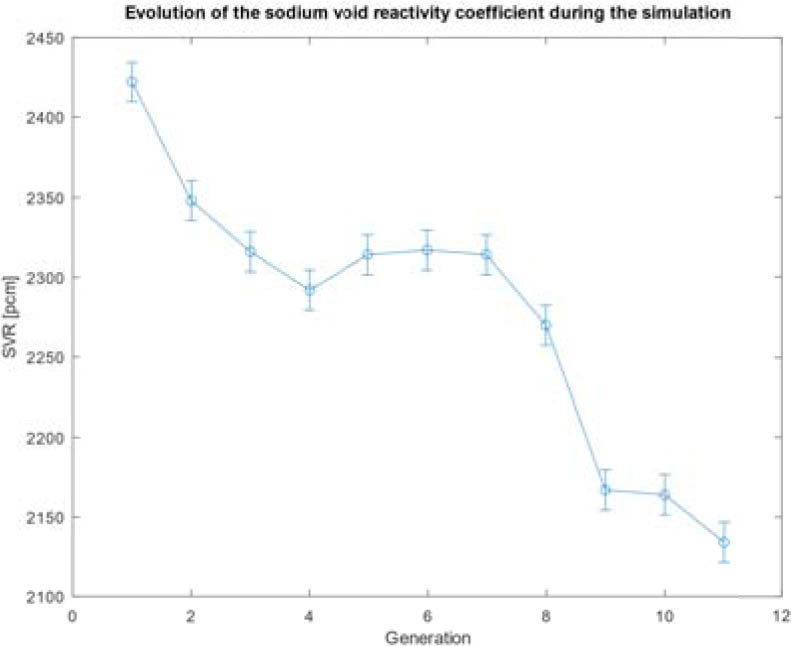
Fig. 4
SVR during the simulation.
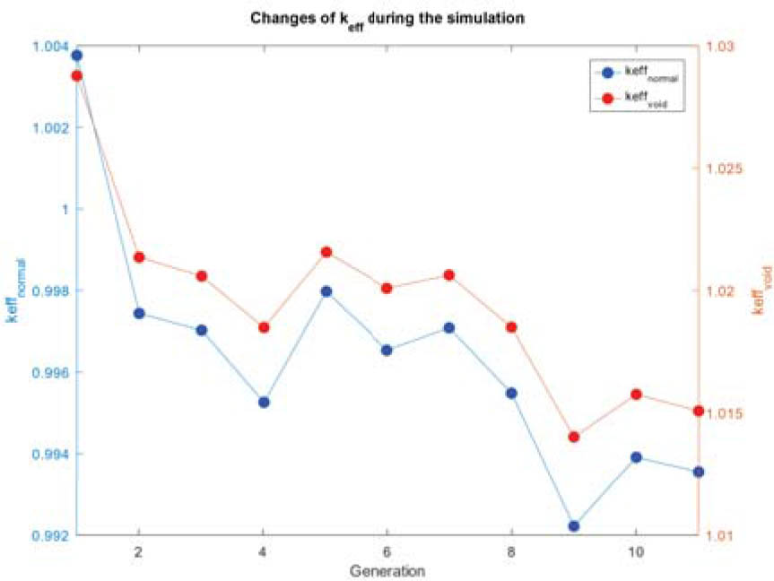
Fig. 5
Eigenvalues during the simulation.
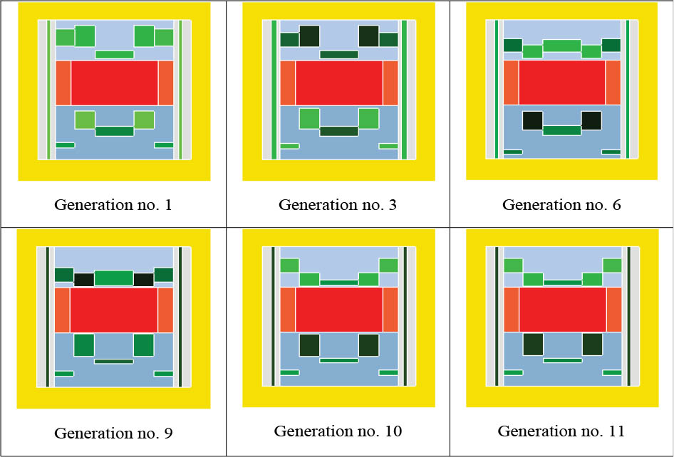
Fig. 6
Changes in the alignment of boron shields in selected generations.
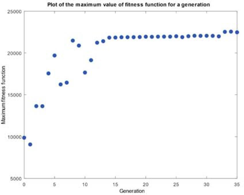
Fig. 7
Maximum fitness function value for each generation.
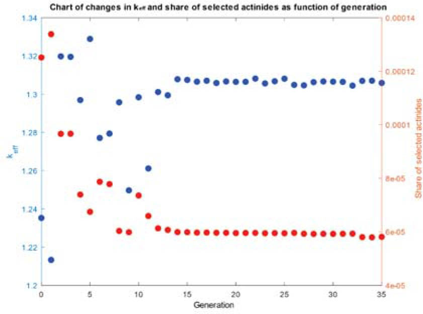
Fig. 8
The eigenvalue and concentration of selected actinides for the best individual in a generation.
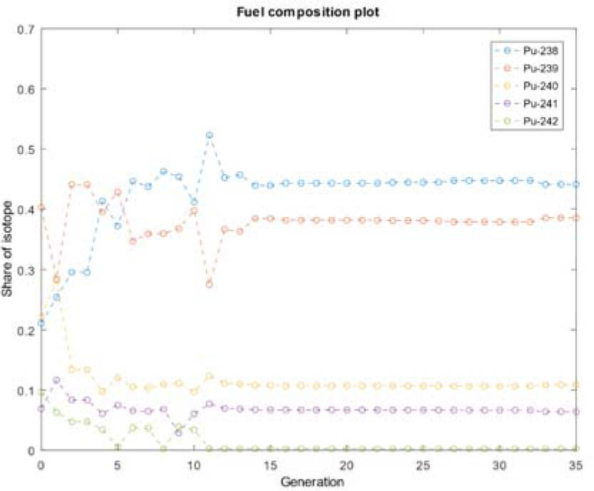
Fig. 9
Isotope composition vs. generations.