
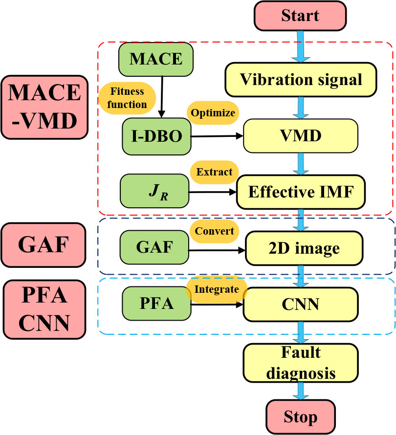
Fig. 1.
Research block diagram.
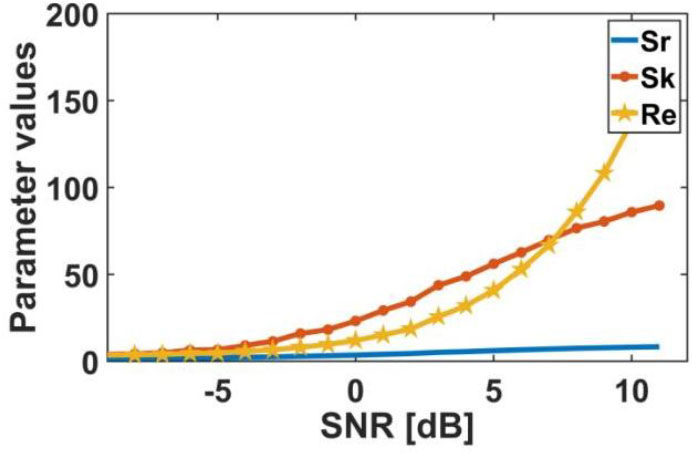
Fig. 2.
Sk, Sr, Re schematic diagram of variation with defects.
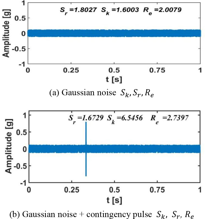
Fig. 3.
Sk, Sr, Re sensitivity to accidental noise.
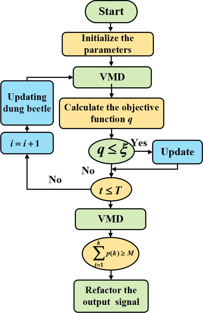
Fig. 4.
Schematic diagram of the variation with defects.
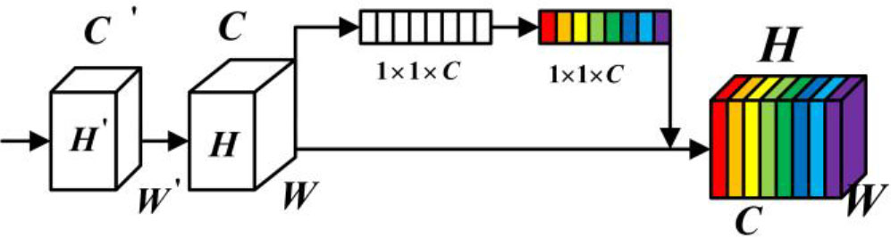
Fig. 5.
Schematic diagram of the channel attention mechanism.
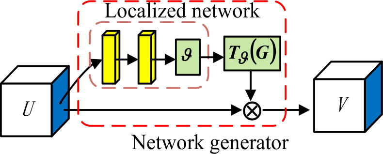
Fig. 6.
Schematic diagram of the spatial attention mechanism.
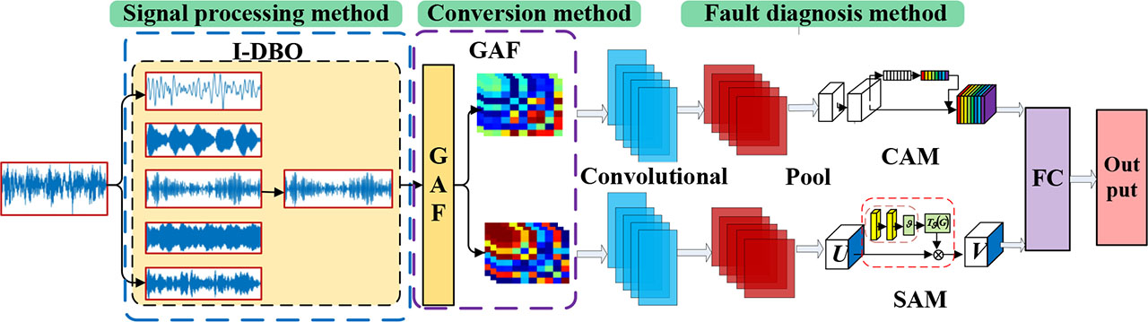
Fig. 7.
MACE + PFACNN model structure diagram.
Table 1.
Experimental parameters.
| Inner diameter [mm] | Pitch diameter [mm] | Thickness [mm] | Outer diameter [mm] | Rolling diameter [mm] | Contact angle [°] |
|---|---|---|---|---|---|
| 25 | 39 | 15 | 52 | 8 | 0 |
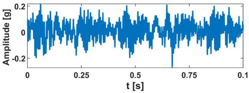
Fig. 8.
Time domain waveform of outer ring signal.
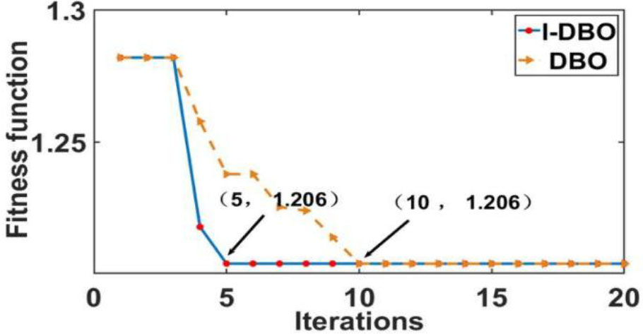
Fig. 9.
Fitness function.
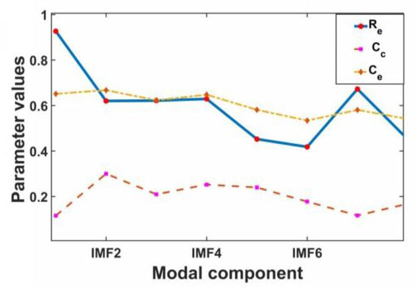
Fig. 10.
Entropy change curve.
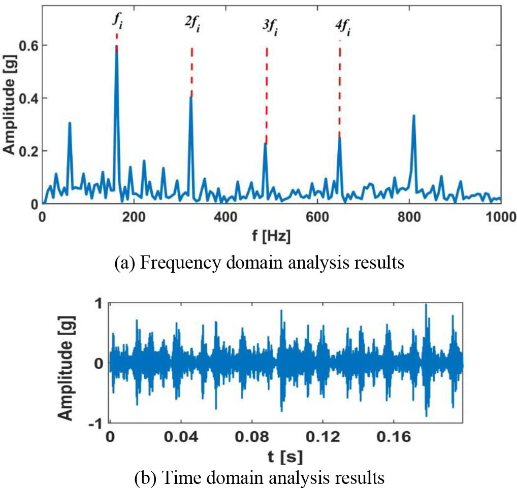
Fig. 11.
Analysis results after MACE-VMD.
Table 2.
Dataset classification.
| Training set | Test set | |||
|---|---|---|---|---|
| Regular | 0 | 1 | 70 | 30 |
| Inner ring | 0.18 | 2 | 70 | 30 |
| 0.36 | 3 | 70 | 30 | |
| 0.54 | 4 | 70 | 30 | |
| Outer ring | 0.18 | 5 | 70 | 30 |
| 0.36 | 6 | 70 | 30 | |
| 0.54 | 7 | 70 | 30 | |
| Rolling body | 0.18 | 8 | 70 | 30 |
| 0.36 | 9 | 70 | 30 | |
| 0.54 | 10 | 70 | 30 |
Table 3.
Fault diagnosis results.
| Category | Accuracy [%] | Category | Accuracy [%] |
|---|---|---|---|
| 1 | 100 | 6 | 100 |
| 2 | 100 | 7 | 100 |
| 3 | 100 | 8 | 99.3 |
| 4 | 100 | 9 | 99.3 |
| 5 | 100 | 10 | 100 |
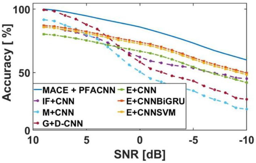
Fig. 12.
Analysis results of noise resistance.
Table 5.
Results of 0 dB white noise comparison test.
| Model | MACE + PFACNN | IF+ CNN | M+ CNN | E+CNN | E+ CNNSVM |
|---|---|---|---|---|---|
| Accuracy [%] | 89.2 | 64.5 | 51.6 | 67.8 | 72.4 |
| Recall rate [%] | 89.8 | 64.9 | 52.1 | 68.2 | 72.9 |
| F1 [%] | 89.7 | 64.6 | 51.8 | 67.7 | 72.6 |
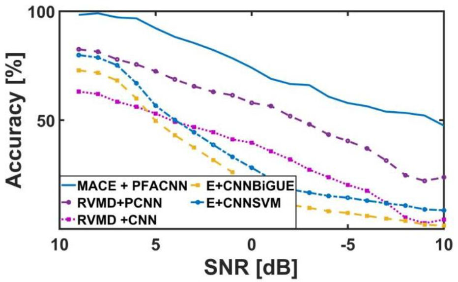
Fig. 13.
Analysis results of the ability to resist complex noises.
Table 6.
Experimental results of 5 dB complex noise comparison.
| Model | MACE + PFACNN | RVMD+ DCNN | RVMD+ CNN | E+CNN BiGRU | E+CNN SVM |
|---|---|---|---|---|---|
| Accuracy [%] | 91.3 | 80.1 | 52.1 | 54.2 | 48.3 |
| Recall rate [%] | 91.6 | 80.5 | 52.7 | 54.9 | 48.8 |
| F1 [%] | 91.4 | 80.3 | 52.5 | 54.6 | 48.6 |
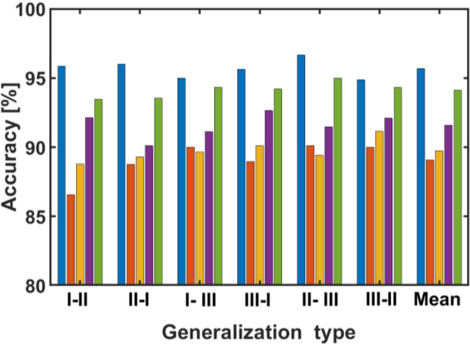
Fig. 14.
Analysis results of the generalization ability.
Table 7.
Generalization experiment results – Accuracy [%].
| Model | MACE + PFACNN | E+CNN | E+SVM | IF+CNN | M+DCNN |
|---|---|---|---|---|---|

|

|

|

|

| |
| I-II | 95.8 | 86.5 | 88.7 | 92.1 | 93.4 |
| II-I | 96.0 | 88.7 | 89.3 | 90.1 | 93.5 |
| I-III | 94.9 | 89.9 | 89.6 | 91.1 | 94.3 |
| III-I | 95.6 | 88.9 | 90.1 | 92.6 | 94.2 |
| II-III | 96.6 | 90.1 | 89.4 | 91.4 | 94.9 |
| III-II | 94.8 | 90.0 | 91.1 | 92.1 | 94.3 |
| Mean | 95.6 | 89.0 | 89.7 | 91.5 | 94.1 |
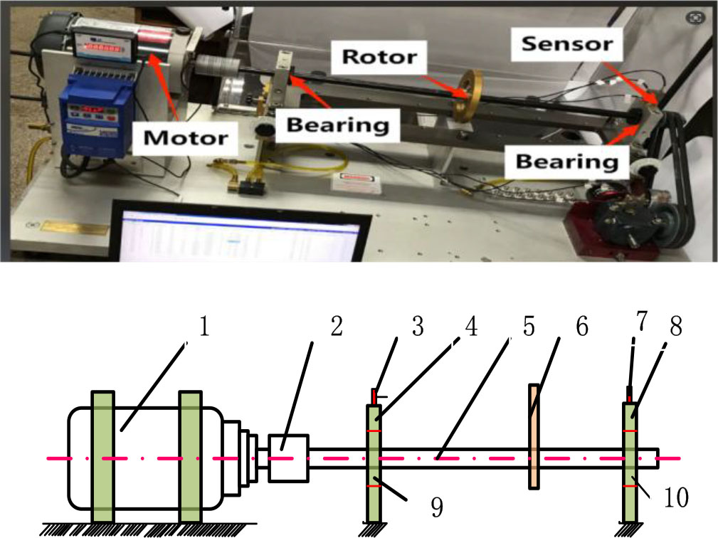
Fig. 15.
Experimental layout.
1. Motor, 2. Coupling, 3. Acceleration sensor, 4. Bearing housing I, 5. Spindle, 6. Rotor, 7. Acceleration sensor, 8. Bearing housing II, 9. Bearing I, 10. Bearing II.
Table 8.
Dataset classification.
| Training set | Test set | |||
|---|---|---|---|---|
| Regular | —— | 1 | 70 | 30 |
| Inner ring | —— | 2 | 70 | 30 |
| Outer ring | 90° | 3A | 70 | 30 |
| 135° | 3B | 70 | 30 | |
| Regular | —— | 4 | 70 | 30 |
| Compound failure | outer 90° | 5A | 70 | 30 |
| outer 135° | 5B | 70 | 30 |
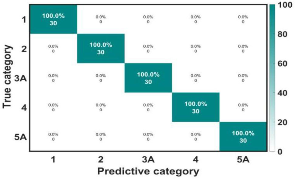
Fig. 16.
Fault diagnosis results.
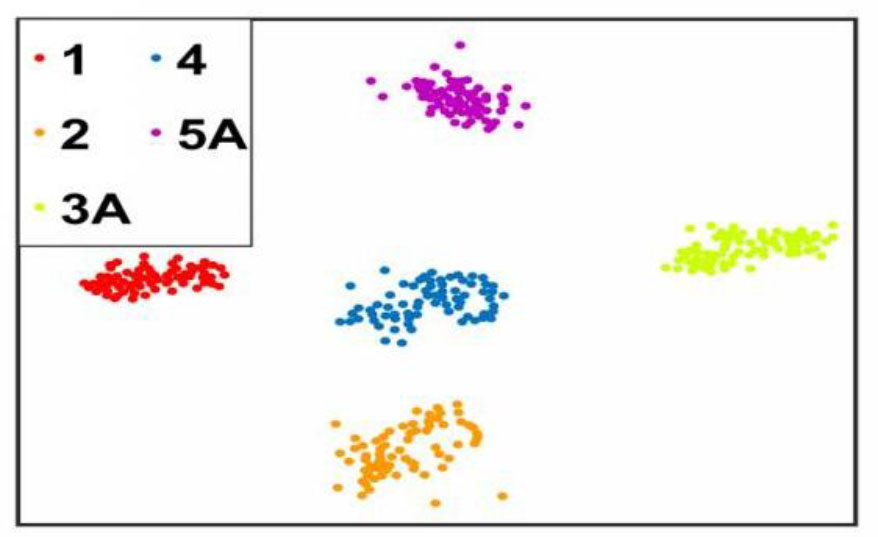
Fig. 17.
Visualization results after diagnosis.
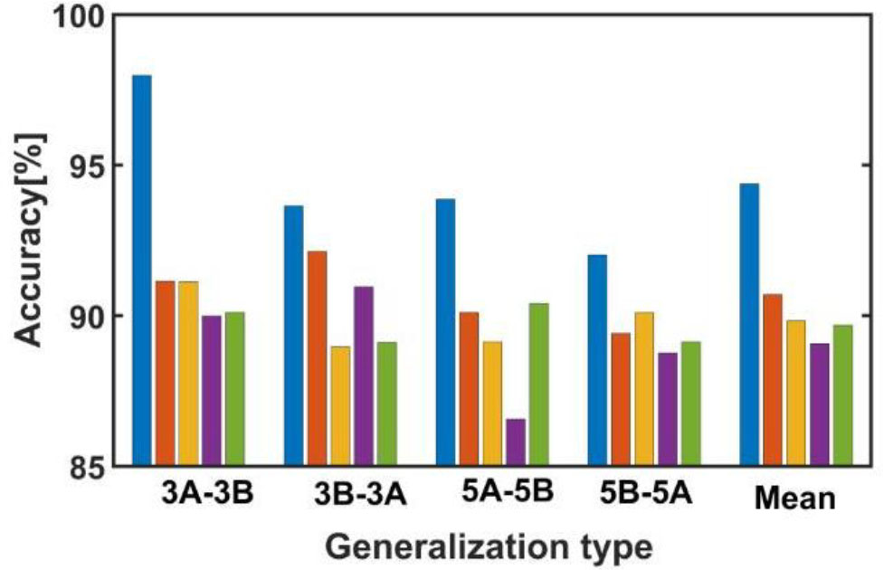
Fig. 18.
Analysis results of generalization ability.


