
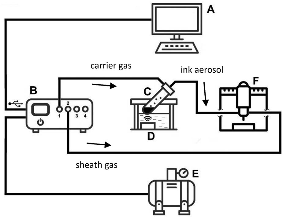
Figure 1
Schematic diagram of the aerosol jet printer with an ultrasonic atomiser equipped with (A) control unit, (B) microfluidic Elveflow controller, (C) ink reservoir, (D) ultrasonic transducer, (E) air compressor, and (F) sonotrode with PH fixed above CNC bed.
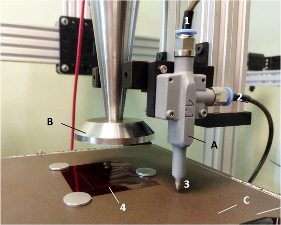
Figure 2
PH (a) and UH (b) fixed and attached to manipulator arm, (c) CNC heating bed. 1 – aerosol inlet, 2 – shielding gas inlet, 3 – exchangeable nozzle with an inner orifice diameter of 0.36 mm, 4 – sample (polyimide foil) with printed traces.
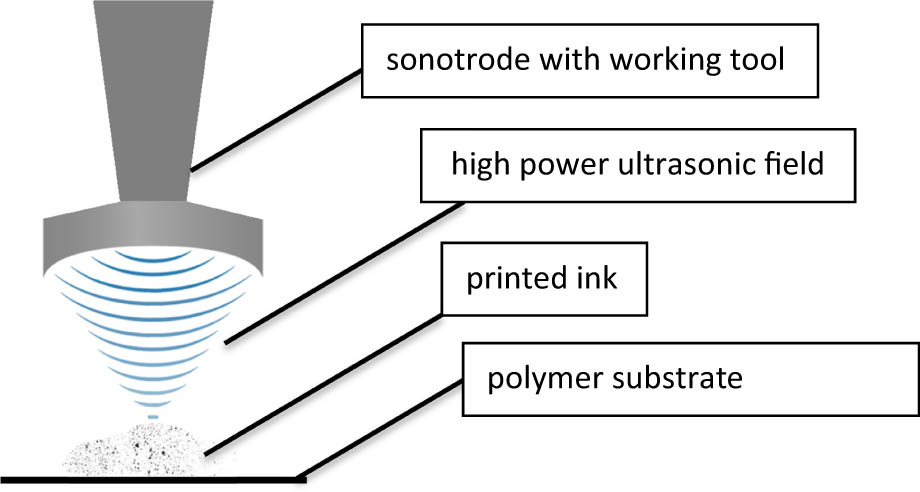
Figure 3
Schematic view of high-power ultrasonic field impact on ink particles.
Table 1
Properties of the utilised ink provided by manufacturer [40].
| Dynamic viscosity (m·Pa·s) | Surface tension (dynes/cm) | Density (g/cm3) | Silver content (%) | Silver powder particle size range (nm) |
|---|---|---|---|---|
| 7.5–10.5 | 28.5–32.5 | 1.1–1.3 | 45 | 3–8 |
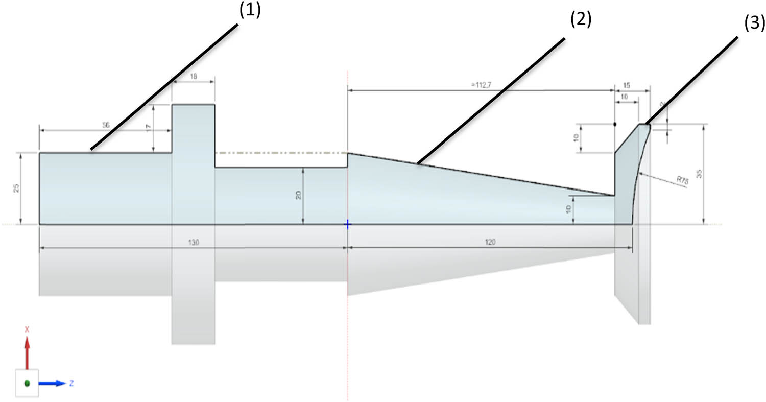
Figure 4
Cross section of the model of the designed ultrasonic system: transducer (1), sonotrode (2), and plate (3).
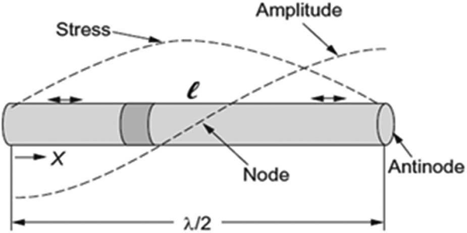
Figure 5
Distribution of vibration amplitude and stress along the waveguide [41].
Table 2
Formulas for estimating length of sonotrode depending on its shape.
| Sonotrode shape | First resonance length |
|---|---|
| Cylindrical | [41] |
| Stepped cylindrical | [42] |
| Exponential | [43] |
| Conical | [44] |
where
| |
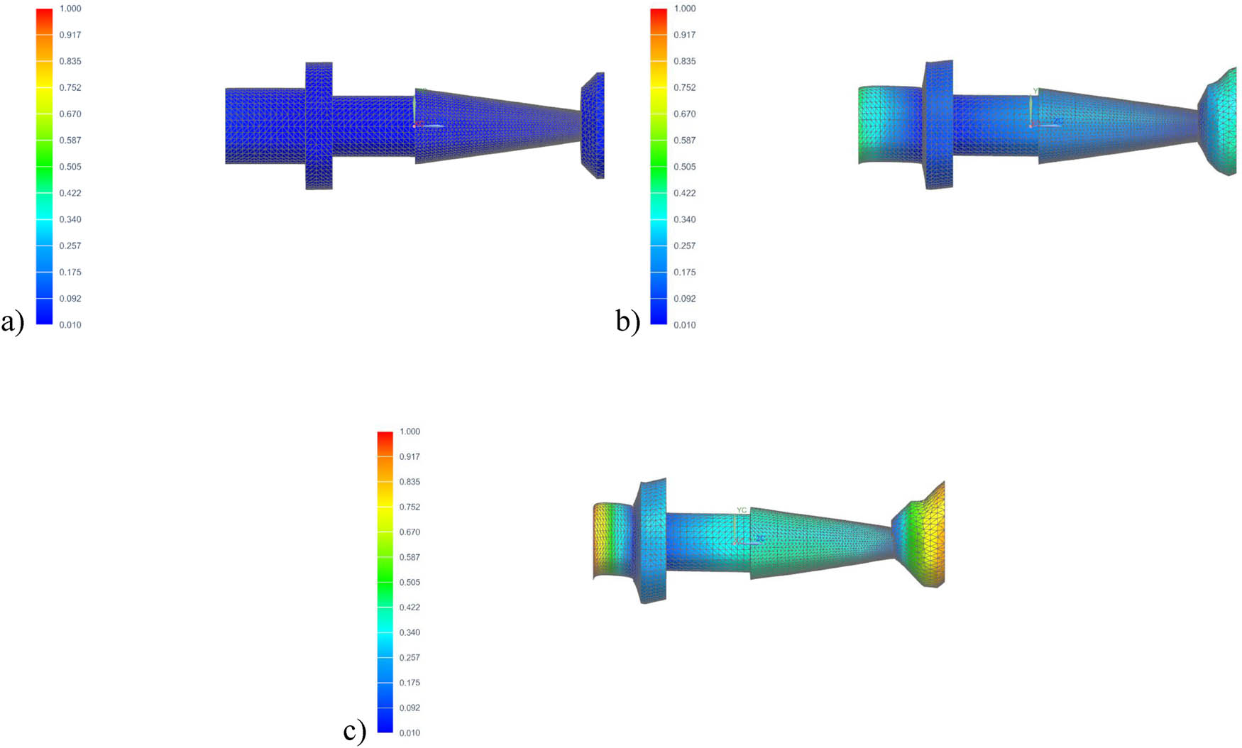
Figure 6
Results of modal analysis of the designed ultrasonic system for 20,000 Hz longitudinal mode. Idle state (a), different phases of tool displacement: +45° (b) and +90° (c).
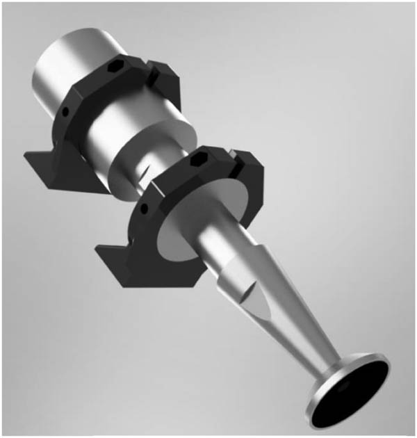
Figure 7
View of 3D model of the ultrasonic system with the working plate for ultrasonic wave concentration.
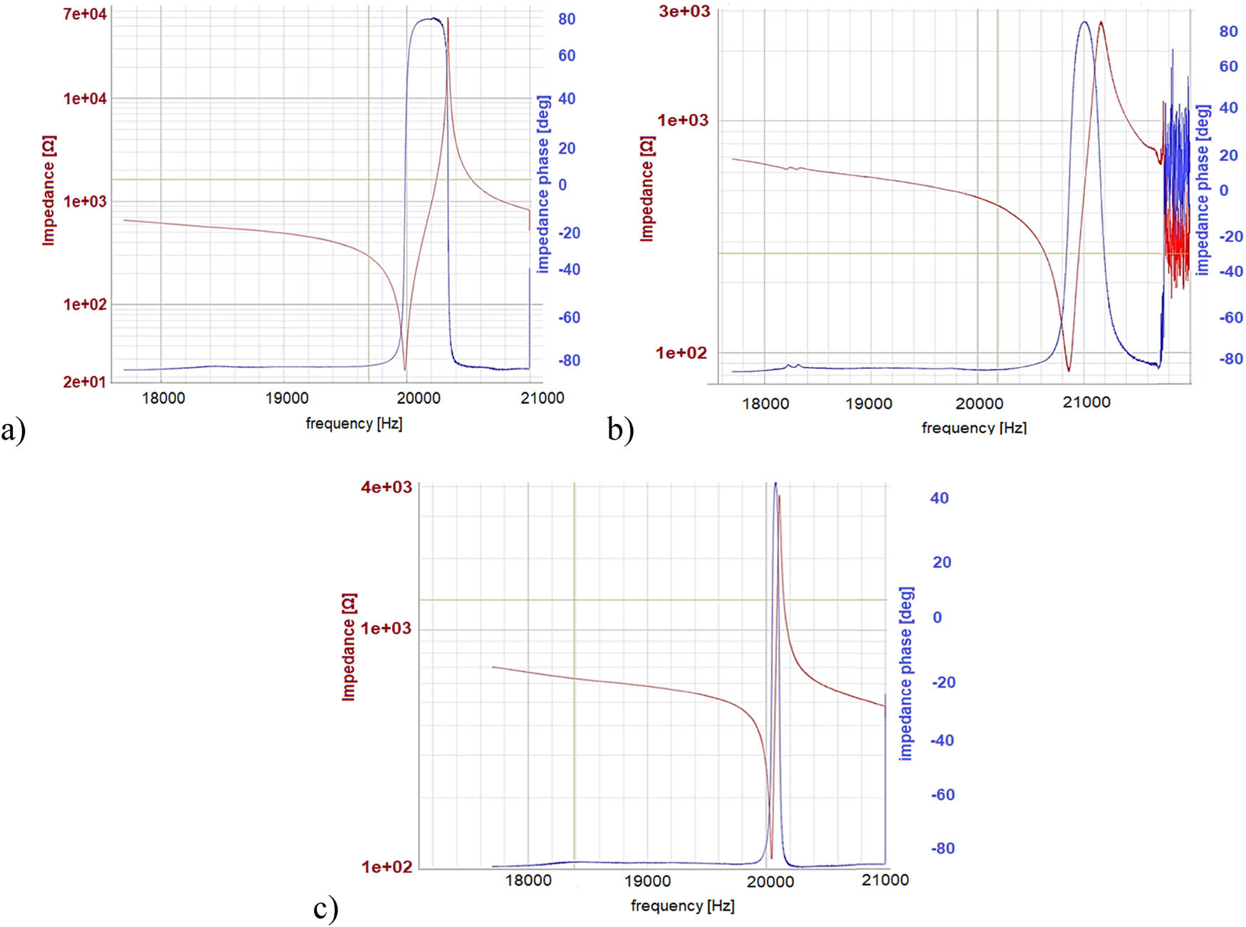
Figure 8
Frequency characteristics of the designed ultrasonic system intended to increase the uniformity of particle distribution of injected paths. Impedance characteristics of transducer (a), transducer coupled with sonotrode (b), and complete ultrasonic system (c).
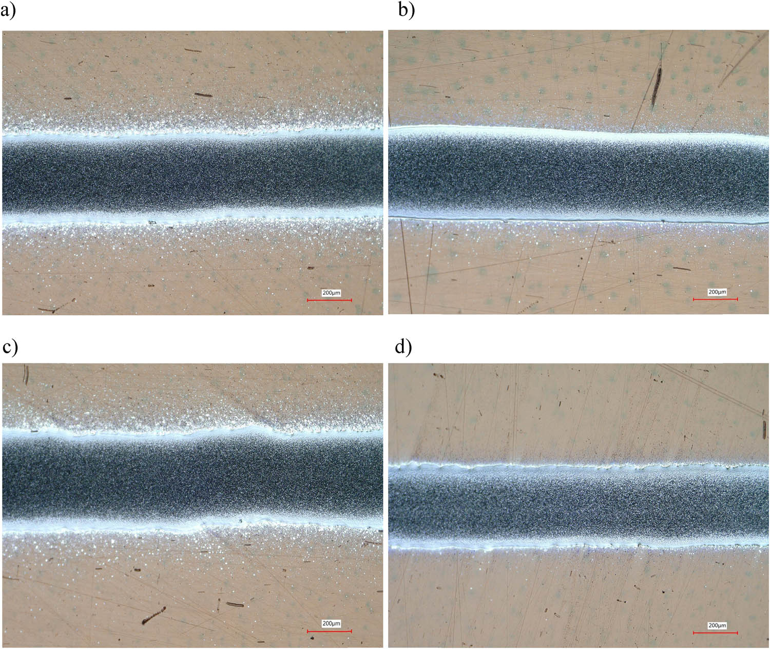
Figure 9
Top view of printed traces: P + S (a), P + H + S (b), P + U + S (c), and P + H + U + S (d).
Table 3
Geometry and properties of printed traces.
| Sample | Width (µm) | Height (nm) | Roughness | SOP (%) | ||
|---|---|---|---|---|---|---|
| Total | Without spilled ink | Average value | Sa (nm) | Sz (nm) | ||
| P + S | 406 ± 8 | 311 ± 11 | 586 ± 31 | 123 ± 20 | 995 ± 33 | 17.2 |
| P + H + S | 383 ± 47 | 294 ± 29 | 556 ± 89 | 91 ± 13 | 888 ± 30 | 9.1 |
| P + U + S | 526 ± 56 | 416 ± 35 | 629 ± 106 | 148 ± 21 | 1158 ± 181 | 5.9 |
| P + H + U + S | 415 ± 29 | 302 ± 33 | 722 ± 103 | 92 ± 9 | 1276 ± 198 | 2.7 |
The values presented in the table contain the standard deviation of the obtained results.
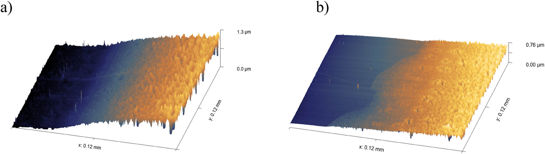
Figure 10
The boundary region of sample P + S (a) and P + U + S (b).
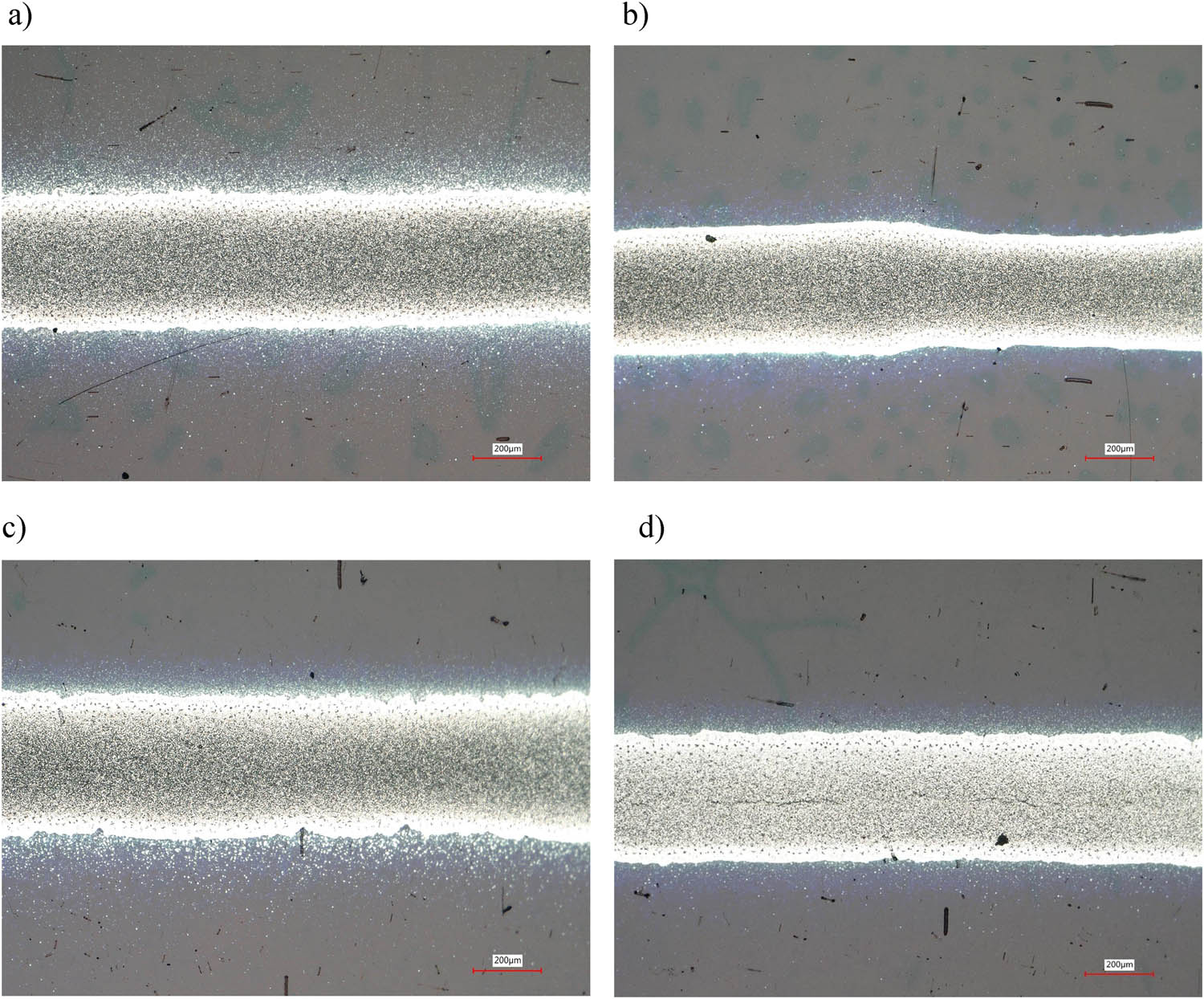
Figure 11
Top view of printed and sintered traces: P + S (a), P + H + S (b), P + U + S (c), and P + H + U + S (d). The dark region in the central part of the trace responds to porosity and high roughness.
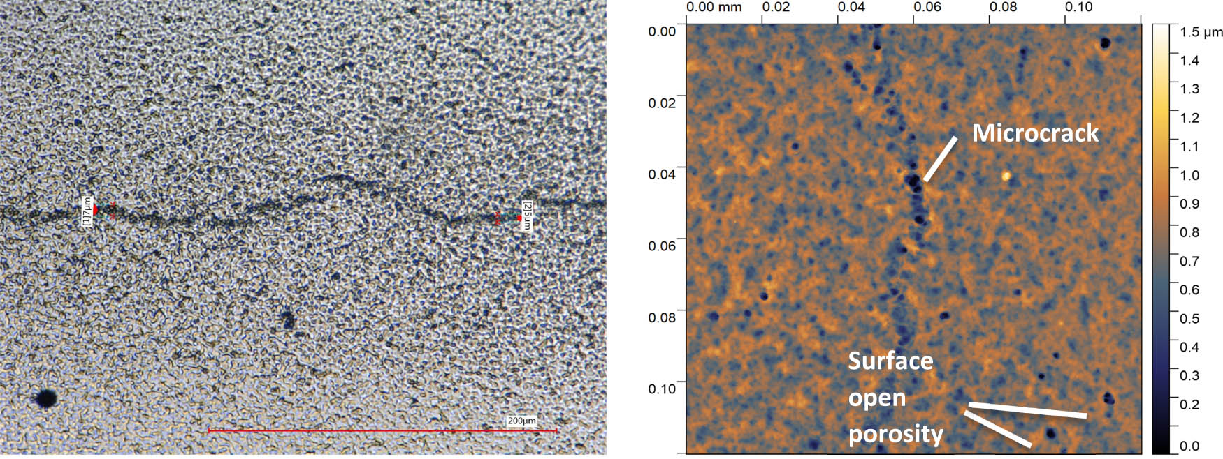
Figure 12
Sample P + H + U + S with a visible crack in the axis: DM (a) and AFM (b).
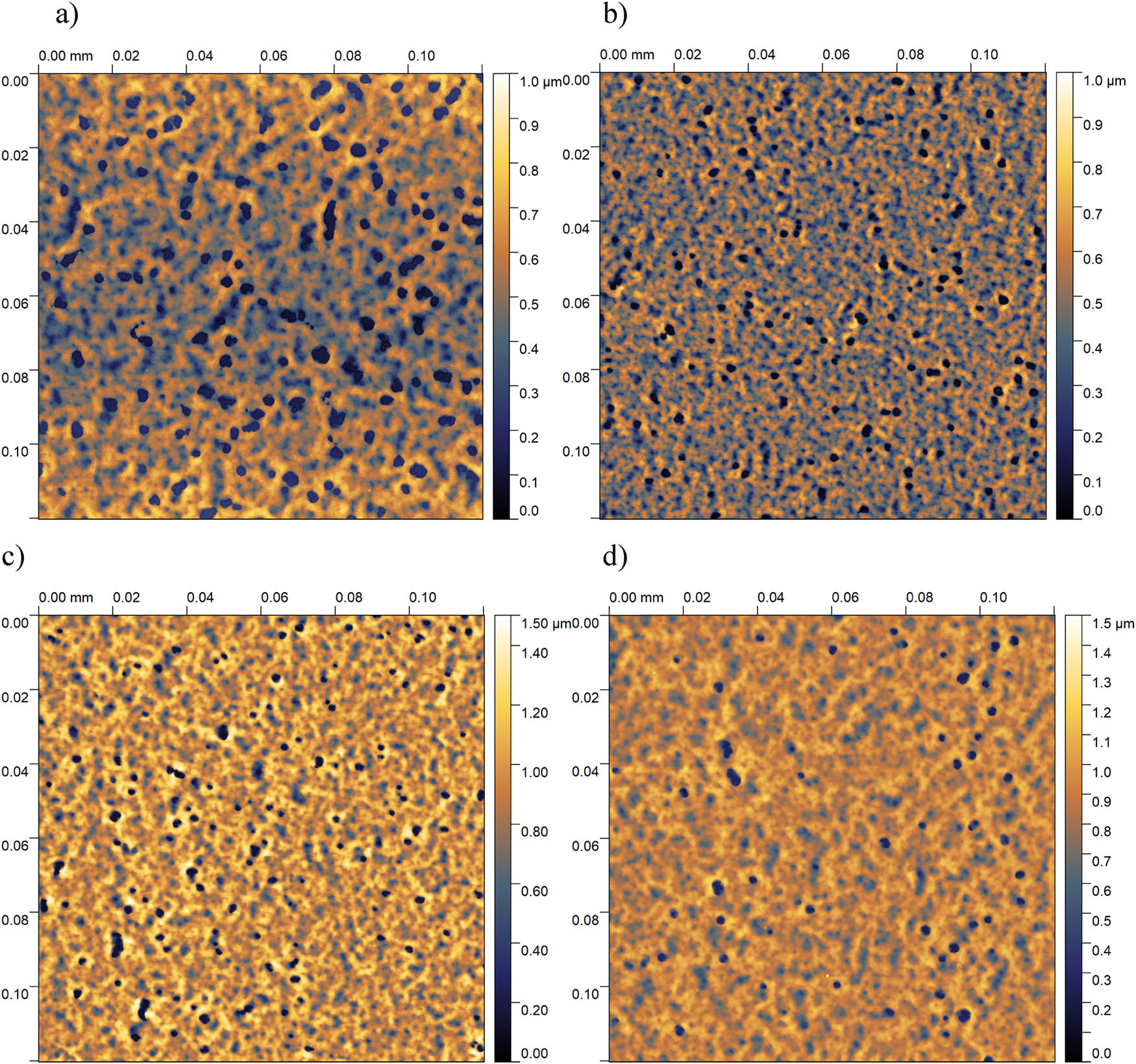
Figure 13
AFM scans of sample surface: P + S (a), P + H + S (b), P + U + S (c), and P + H + U + S (d). Black dots respond to SOP.
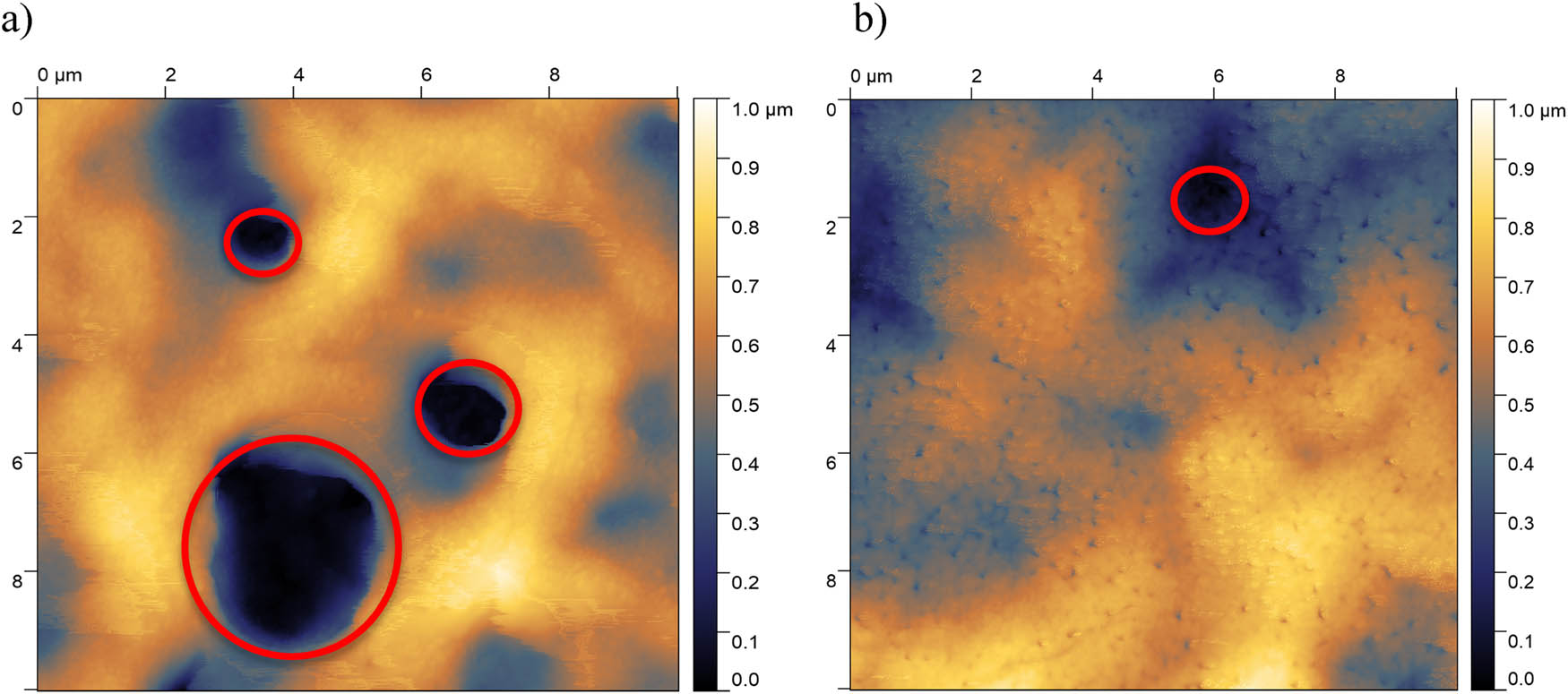
Figure 14
AFM micrographs of P + S (a) and P + U + S (b) samples. Red circles highlight black dots and respond to SOP.
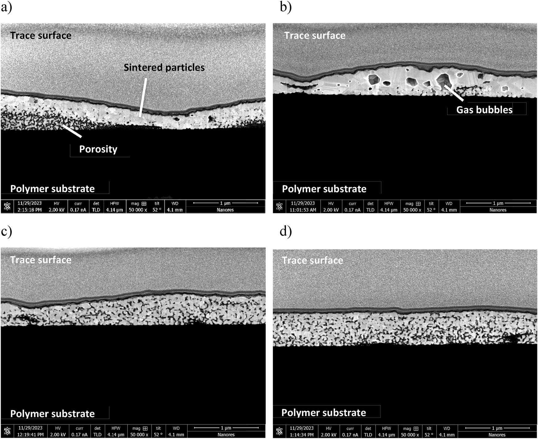
Figure 15
SEM micrographs presenting cross-section of printed traces: P + S (a), P + H + S (b), P + U + S (c), and P + H + U + S (d).
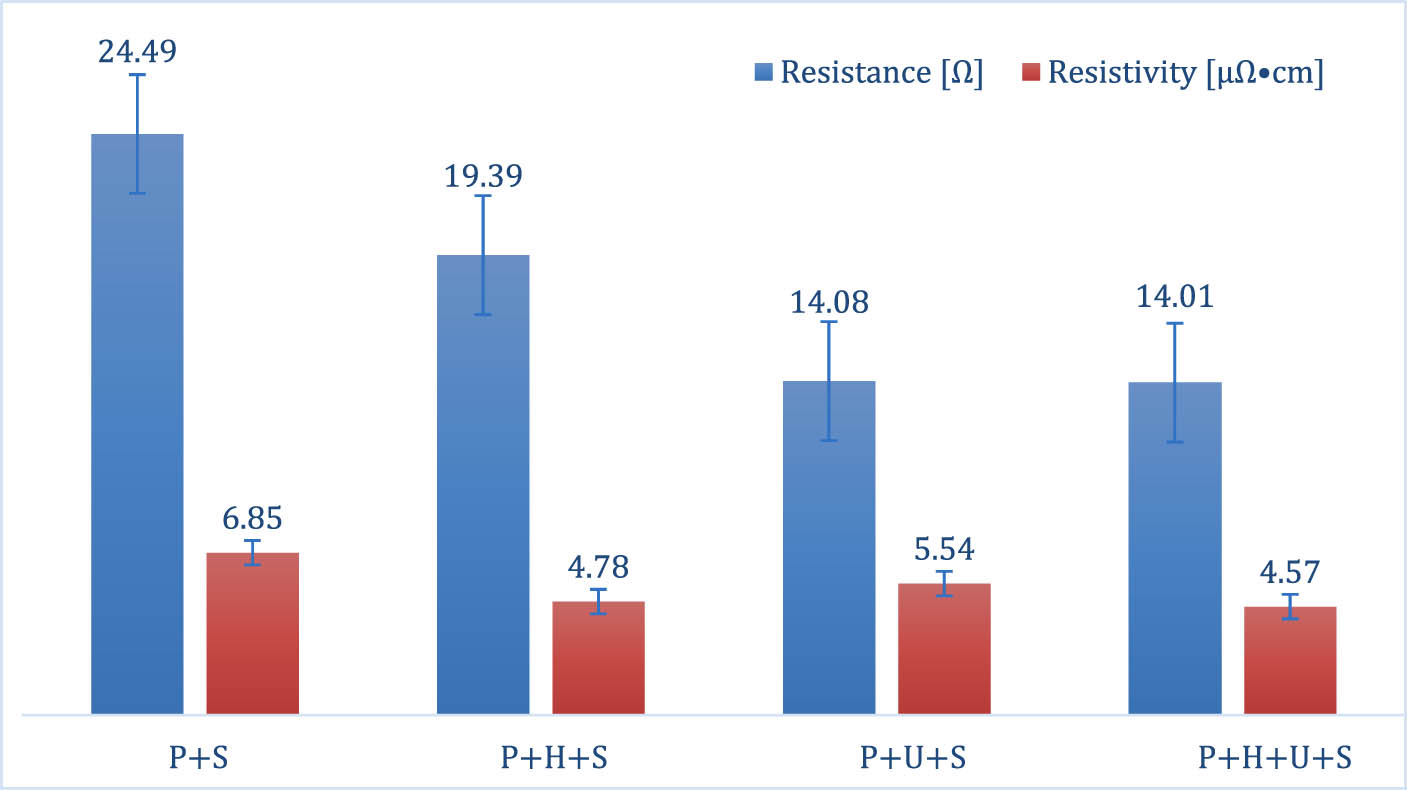
Figure 16
Results of resistance measurements and resistivity calculations.