
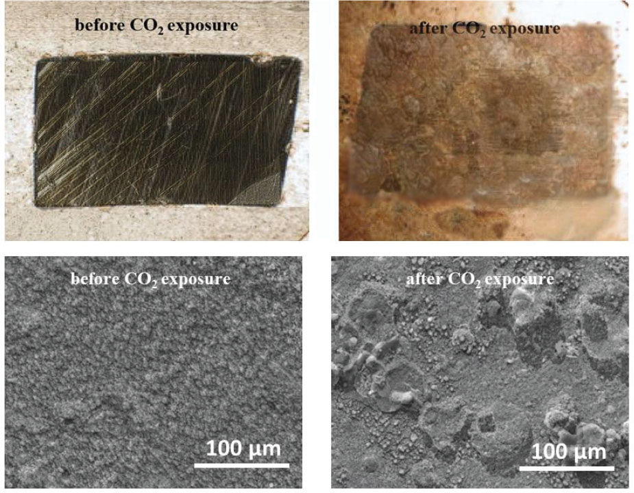
Fig. 1.
Binocular photographs and SEM image of N80 steel surface before and after CO2 exposure
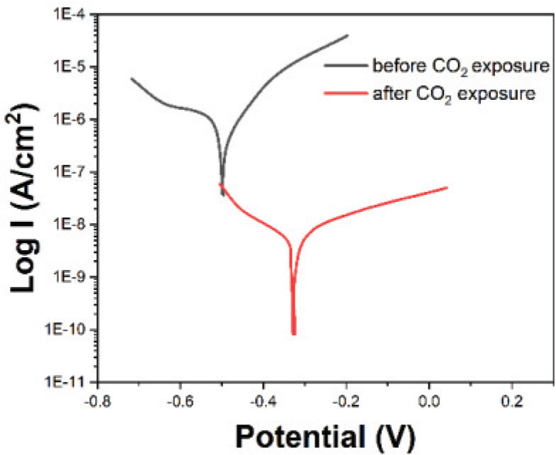
Fig. 2.
Potentiodynamic polarization curves for N80 steel
Table 1.
Summary of EIS measurements for N80 steel
| Sample | Rel+b (kΩ/cm2) | Qpn, | n | Rpn (kΩ/cm2) | Qpn, | n | Rct (kΩ/cm2) |
|---|---|---|---|---|---|---|---|
| Before CO2 exposure | 84.03±3.20 | 5.78E−09±2.89E−10 | 0.5708±0.0285 | 30.24±1.21 | 1.05E−04±5.25E−06 | 0.6877±0.0344 | 355.21±14.21 |
| After CO2 exposure | 22.24±0.89 | 2.53E−09±1.26E−10 | 0.5541±0.0277 | 2.99±0.12 | 1.73E−03±8.65E−05 | 0.8153±0.0408 | 200.40±8.02 |
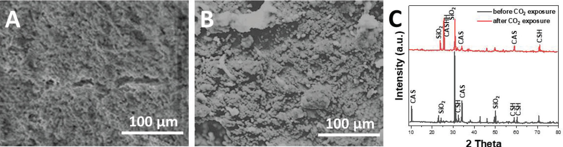
Fig. 3.
SEM image of (A) unexposed and (B) post-exposure cement paste. (C) XRD patterns of cement paste before and after CO2 exposure
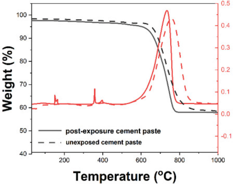
Fig. 4.
TGA curves for unexposed and post-exposure cement paste
Table 2.
Nano-indentation test results for cement paste
| Exposure Duration (Months) | Hardness (GPa) | Elastic Modulus (GPa) | Indentation Depth (μ m) |
|---|---|---|---|
| 0 (Control) | 1.25±0.04 | 25.0±0.36 | 2.50±0.04 |
| 1 | 1.15±0.03 | 23.8±0.65 | 2.65±0.07 |
| 2 | 1.05±0.07 | 22.6±0.44 | 2.80±0.03 |
| 3 | 0.95±0.03 | 21.4±0.27 | 2.95±0.08 |
| 4 | 0.85±0.04 | 20.2±1.03 | 3.15±0.11 |
| 5 | 0.75±0.05 | 19.0±0.85 | 3.30±0.09 |
| 6 | 0.65±0.06 | 17.8±0.78 | 3.50±0.14 |
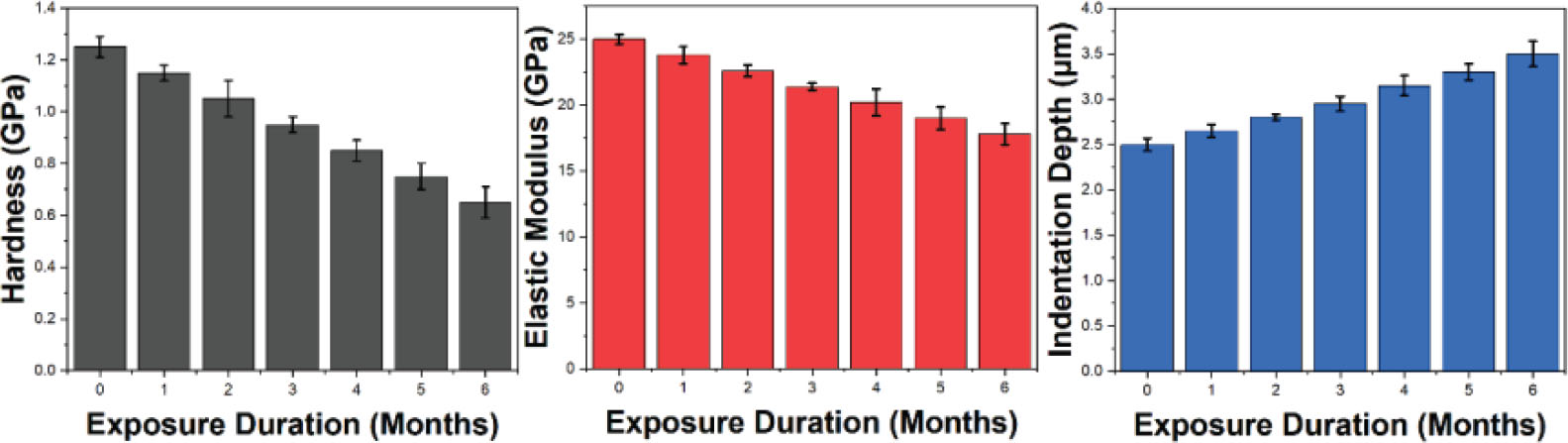
Fig. 5.
Nano-indentation test results for cement paste
Table 3.
Ultrasonic Testing results for the steel-cement interface
| Exposure Duration (Months) | Acoustic Impedance (MRayl) | Velocity of Sound (m/s) | Signal Amplitude (dB) |
|---|---|---|---|
| 0 (Control) | 45.0±4.3 | 5940±80 | −12.5±0.5 |
| 1 | 43.5±3.2 | 5720±70 | −10.4±0.3 |
| 2 | 42.7±1.5 | 5610±60 | −9.7±0.4 |
| 3 | 40.0±3.2 | 5570±60 | −8.5±0.5 |
| 4 | 38.5±2.4 | 5550±70 | −7.2±0.4 |
| 5 | 36.2±2.0 | 5430±80 | −6.5±0.3 |
| 6 | 34.1±1.4 | 5370±50 | −5.9±0.4 |
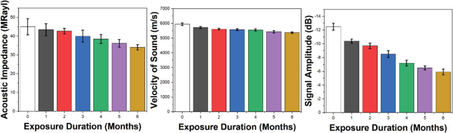
Fig. 6.
Ultrasonic testing results for the steel-cement interface
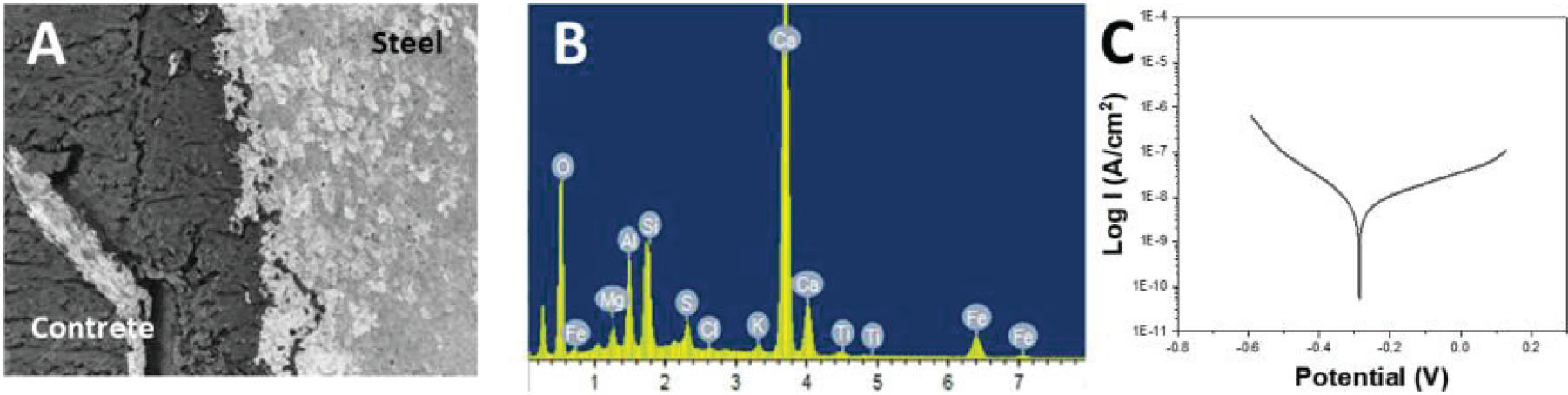
Fig. 7.
(A) SEM image and (B) EDX spectrum of the steel-cement interface after CO2 exposure. (C) potentiodynamic polarization curves at the steel-cement interface
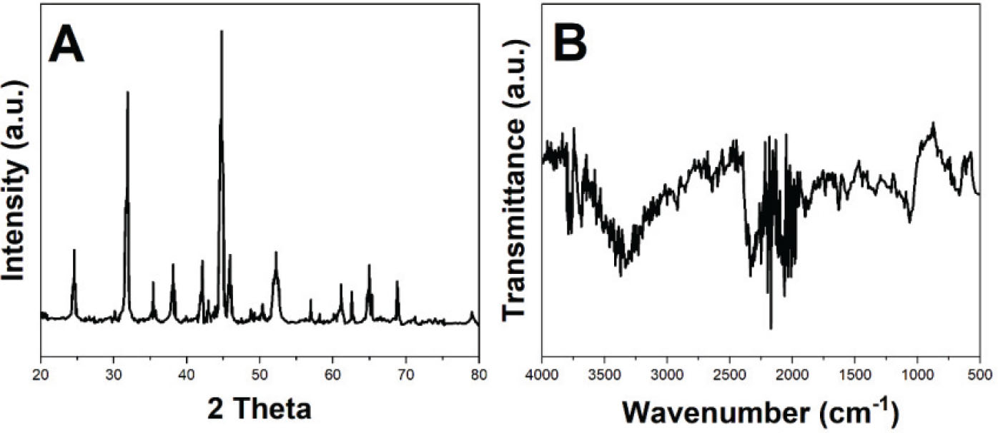
Fig. 8.
(A) XRD patterns showing corrosion products on N80 steel. (B) FTIR spectra of degraded layers on N80 steel
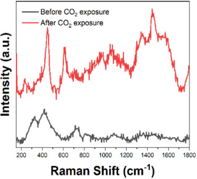
Fig. 9.
Micro-Raman spectra of the interface region
Table 4.
Electrochemical parameters of steel at the interface
| Exposure Duration (Months) | Corrosion Potential (mV, SCE) | Corrosion Current Density (μA/cm2) | Polarization Résistance (kΩ/cm2) |
|---|---|---|---|
| 0 (Control) | −453±13 | 0.5±0.03 | 20±0.4 |
| 1 | −472±11 | 0.8±0.04 | 18±0.6 |
| 2 | −497±10 | 1.2±0.03 | 16±0.7 |
| 3 | −514±7 | 1.6±0.04 | 13±0.5 |
| 4 | −532±11 | 2.1±0.03 | 10±0.9 |
| 5 | −553±14 | 2.7±0.02 | 8±0.7 |
| 6 | −572±7 | 3.4±0.03 | 5±0.8 |
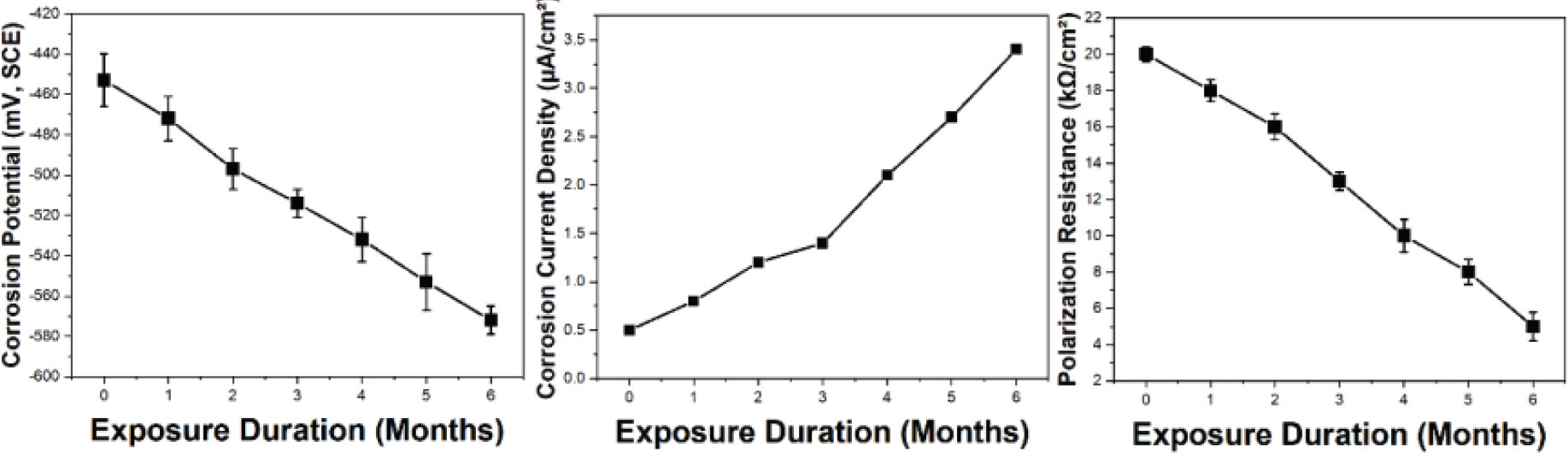
Fig. 10.
Electrochemical parameters of steel at the interface
Table 5.
ICP-MS results showing ion flux in CO2 environments
| Exposure Duration (Months) | Iron Concentration (ppm) in Brine | Calcium Concentration (ppm) in Brine | Silicon Concentration (ppm) in Brine |
|---|---|---|---|
| 0 (Control) | 0.5±0.08 | 1.2±0.12 | 0.8±0.05 |
| 1 | 1.1±0.07 | 1.8±0.09 | 1.2±0.08 |
| 2 | 2.0±0.09 | 2.5±0.30 | 1.7±0.05 |
| 3 | 3.2±0.12 | 3.5±0.25 | 2.3±0.06 |
| 4 | 4.5±0.22 | 4.8±0.33 | 3.1±0.07 |
| 5 | 5.9±0.21 | 6.2±0.51 | 4.0±0.12 |
| 6 | 7.5±0.43 | 7.9±0.34 | 5.2±0.44 |
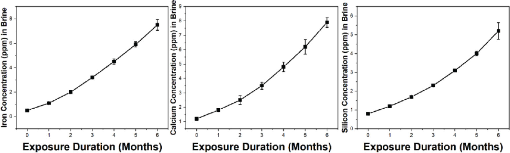
Fig. 11.
ICP-MS results showing ion flux in CO2 environments