
The delivery system refers to a range of methods for delivering any medicine into the human body. Medicines are never administered in their pure form but should be formulated in a suitable delivery system [1]. According to the rate of drug release, the drug delivery system is divided into two main categories: conventional and controlled delivery systems. The conventional delivery system usually provides a rapid drug release over the treatment period. Hence, patients are required to take multiple doses over their treatment period, and so this delivery system is suitable in the case of short-term treatment. On the other hand, the controlled delivery system provides a slow drug release over the treatment period, and thus there is no need for multiple daily dosing. It is also a good option for treating chronic diseases; this leads to an improvement in the adherence of patients to their medicines [2].
The conventional delivery system of any medicine can be modified using several methods. One of the methods is known as nanoparticles (NPs) technology. NPs technique is one of the nanotechnology sciences that provide many advantages in treating chronic diseases by controlling delivery systems [3]. Schizophrenia is a chronic disease affecting 20 million people worldwide, and the annual number of new cases is estimated at 1.5%/10,000 people [4, 5]. According to the Schizophrenia and Related Disorders Alliance of America [6], schizophrenia affects around 1.1% of the world’s population, and the most recent reports indicated that 3.5 million people in the US alone are diagnosed with schizophrenia [5]. Another report indicated that around 1.2% of Americans suffer from schizophrenia [7]. The conventional delivery systems of schizophrenia’s medicines are usually associated with some undesirable side effects like uncontrollable movements, muscle construction, and tremors [8]. Most patients do not respond or partially respond to the current conventional drug delivery system [9]. It is estimated that 30% of schizophrenia patients do not respond adequately to the available drug treatments [10]. A recent review revealed that 49% of patients with schizophrenia were not in adherence to their medications [11]. However, non-adherence of patients to the current medicines are mainly due to the potential side effects and high dose frequency [12].
Fluphenazine (FZN) is a medicine that is effectively used for chronic schizophrenia [13]. FZN is given in two to four divided doses [14, 15]. The FZN conventional delivery system is associated with some undesirable adverse effects [16]. Thus, the need to reduce frequent daily dosing and the side effects associated with the FZN conventional delivery system is becoming urgent.
In this work, FZN (for schizophrenics) has been utilized as a model for modifying its delivery system to be controlled using NPs technology. In this context, the holistic approach in any experimental design utilizes the DoE instead of the traditional approach (i.e., OVAT) to conserve resources [17].
DoE is a well-established approach for designing and conducting experiments and is used in many applications. Experimental designs can be categorized into three main design models: mixture, process or factorial, and mixture-process designs. The mixture model is used when the components are dependent on each other, and changing the proportion in one component spontaneously affects the proportion of other components, since the sum of proportions must be 1. However, the mixture DoE approach was employed in NPs applications. For instance, the mixture DoE approach has been utilized to optimize an aerosolized nanoemulsion system containing docetaxel and curcumin [18]. The authors have identified five components in the mixture, which were (X–1–: safflower seed oil), (X–2–: lecithin), (X–3–: Tween 85: Span 85), (X–4–: Glycerol), and (X–5–: Water), to investigate two responses: (Y–1–: particle size) and (Y–2–: volume median diameter); 24-runs were generated accordingly.
The second category in DoE is factorial design. This category is used for process development when the defined variables are not dependent on each other. This design approach has also been applied in many previous studies in NPs applications. For example, the factorial DoE approach has been applied to optimize the drug delivery system of olanzapine in polymeric NPs [19]. Another study suggested a mathematical model for fabricating methotrexate to load it in chitosan (CS) NPs by utilizing factorial DoE [20]. Besides, factorial design (32) and statistical analysis were carried out to develop the zolmitriptan nanoparticulate drug delivery system (drug-loaded in CS polymer) [21].
The third category is mixture-process design. This design is utilized when it is essential to investigate the relationship between the proportion of components and process parameters [22]. This design is also utilized in pharmaceutical applications. For example, the hardness of tablets during the manufacturing process was optimized using the mixture-process DoE approach [23]. Three components were identified in that mixture with some constraints [i.e., X–1–: is a binder (formed 4–8% of the mixture), X–2–: is a lubricant (formed 1–3% of the mixture), and X–3–: is a disintegrant (formed 1–3% of the mixture)]. Ninety percent of the mixture contains the active ingredient, and the remaining components (i.e., X–1–, X–2–, and X–3–) form 10% of that mixture. Besides, two process variables were identified in the model [i.e., particle size (Z–1–) and mixing time (Z–2–), with the constraints of (0.5–1) and (5–10), respectively].
Accordingly, choice one of the above DoE approaches depends on the nature of the case study. Since this study aimed to investigate the relationship between the mixture [i.e., FZN, CS, and tripolyphosphate (TPP)] and process variables (i.e., mixing time and pH), the mixture-process design approach was employed to design the experimental work. Besides, some constraints on the identified variables make the mixture-process DoE the best approach for building a design space [23].
In the optimization phase, finding one solution that simultaneously optimizes objectives could be complicated without conflict among the objectives [24]. Thus, we usually look for “trade-offs” rather than a single solution in multiobjective optimization (MOO) cases. Classical approaches for optimizing multiobjective cases are either the scalarization approach or the heuristic approach. The scalarization optimization approach sums all objectives in a single objective using predefined weights [25]. On the other hand, the heuristic optimization approach is widely employed for solving engineering design problems, and in the drug discovery field as well [26], because this approach does not need any derivatives of the objective function to find the optimum solution, whereas computer codes calculate numerical values corresponding to multiple objectives and constraints. Besides, heuristic optimization methods are more likely to find a global optimum and are not trapped around local optima during the search. A genetic algorithm is a non-derivative method that is well-fit to solve highly combinatorial cases [27].
Multiobjective evolutionary algorithms (MOEA) have been recently applied in numerous applications, due to their adequacy and strength in providing a set of optimal solutions between divergent and non-measurable goals [28]. One of the most efficient algorithms for solving MOO problems is the non-dominated sorting genetic algorithm (NSGA). This algorithm has two versions NSGA-I and NSGA-II. The primary algorithm in NSGA-I was introduced to improve the elitism approach, which involves keeping the generations through the evolutionary process [29]. NSGA-II (Pareto front) uses a different approach, rather than the weighted coefficients approach in the classical optimization techniques; it involves the sorts of points generated by changing the coefficients [30].
In the literature, a study utilized NSGA-II to optimize nanofluid’s mixture-process model [30]. The authors have identified thermal conductivity and viscosity as the study objectives by maximizing thermal conductivity and minimizing viscosity. NSGA-II was utilized to provide an optimum combination of two parameters (temperature and volume fraction of nanocomposite) after generating two equations related to the responses. Optimum solutions have been generated as a set of solutions (Pareto front). In the end, one solution of the Pareto front has been selected as the trade-off points.
NSGA-II has also been utilized as a methodology to optimize the thermal and rheological properties of aluminum NPs [31]. The authors have optimized four objectives (convective heat transfer, viscosity, thermal conductivity, and heat capacity). Artificial neural network (ANN) and response surface methodology (RSM) were used to build the mathematical models based on two variables (temperature and NPs concentration). The Pareto front was generated accordingly.
Furthermore, the NSGA-II approach has been introduced in the pharmaceutical supply chain field. For example, NSGA-II has been utilized in optimizing the three objectives (i.e., manufacturing costs, product quality, and environmental affect through transportations) that apply to determination of the parameters involved in pharmaceutical supply chains [32]. In that study, many parameters were included in the model, such as suppliers, plants, hospitals, collection centers, recycling centers, disposal centers, raw materials, drug type, and periods. NSGA-II algorithm parameters were 0.3, 0.7, 30, and 75 for mutation rate, crossover rate, population size, and iteration size, respectively. In the end, NSGA-II has been successfully able to provide optimum solutions when dealing with that complicated model.
In another study, NSGA-II solved the MOO problem in NPs applications [33]. In that study, authors have utilized an ANN to propose a mathematical model between the input variables (PLGA molecular weight as polymer, PLGA concentration, rate of sonication, and molecular weight of PVA as a stabilizer) and two responses (PLGA particle size and release behavior). NSGA-II algorithm was used to optimize NPs formulation and provide a Pareto front with minimum particle size and perfect release pattern.
This study aims to develop a mathematical model for FZN to optimize its (FZN-CSNPs) nanocomposite delivery system using a mixture-process involving DoE and MOO approaches. Optimizing FZN by delivering it through its nanocomposite can also provide a sustained drug release with a constant bloodstream medicine level. Thus, multiple daily doses of FZN might be reduced, and adherence to treatments among patients would be improved accordingly.
NSGA-II will be carried out for optimization procedure to generate the objective functions of optimal fitness value. To the authors’ best knowledge, utilizing multiple statistical analysis tools [DoE-mixture, analysis of variance (ANOVA), and regression analysis] and MOO method (i.e., NSGAII) in fabricating FZN-CSNPs nanocomposite has not been addressed yet in the literature. In this study, four NPs input fabrication parameters were identified as FZN percentage (i.e., FZN), CS percentage (i.e., CS), TPP percentage (i.e., sodium TPP), and pH. Those parameters’ influences were evaluated in terms of the following three responses through this study: NPs size, zeta potential (ZP) (i.e., ZP), and loading efficiency (LE%) [i.e., drug (LE)].
This work required seven main stages to solve the problem and meet the objectives. These stages are summarized in Figure 1.
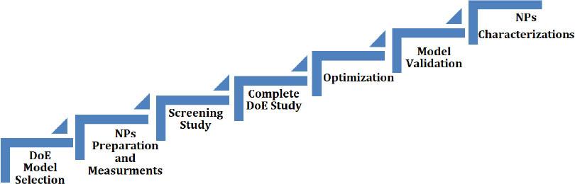
Methodology flow chart. NPs, nanoparticles
An extreme vertices mixture-process DoE was utilized in modeling all experimental work (screening study and complete DoE) for the following reason: NPs fabrication process contains three components (FZN, CS, and TPP) with two process variables (pH value and mixing time). The model utilized is constrained with the following conditions:
FZN, CS, TPP ≠ 0
FZN = (range of 5.0–15.0%, FZN ≠ 0)
CS = (range of 22.5–72.5%, CS ≠ 0)
TPP = (range of 22.5–72.5%, TPP ≠ 0)
FZN + CS + TPP = 100.0%
The primary chemical materials used in this research were fluphenazine deaconate (FZN) (a gift from Hikma Pharmaceutical Inc., lot No. RAC163USP0FC, purity of 99%), CS (low molecular weight 10–120 kDa, 90% deacetylation, lot No. STBH7664) by Sigma-Aldrich (Taufkirchen, Germany), and sodium TPP by AZ Chemical Inc. (lot No. 1161/1162). All other chemical materials, including acetic acid, acetone, sodium hydroxide (NaOH), acetonitrile, methanol, and ammonium acetate, were purchased from Sigma-Aldrich.
The nanocomposite was fabricated using a well-known process called ionotropic gelation (IG). This IG procedure was first developed by Calve [34]. Through ionic interaction between CS with a positive charge of the amino acid group and TPP with a negative charge of a phosphate group, it forms gels [35]. The NPs are formed accordingly by mixing the mixture in a specific range of proportions for each starting material.
In this study, the first step in fabricating (FZNCSNPs) was to separately prepare the three solutions (i.e., CS, TPP, and FZN). The CS was dissolved in 2% w/v acetic acid solution to form CS solutions of 0.5–1.6% w/v. The TPP was dissolved in 50 mL water to form solutions of 1.0–3.2% w/v, whereas FZN was dissolved in 20 mL acetone to form solutions of 0.6–1.7% w/v. The second step was adding the FZN solution over the CS solution gradually using a burette. The last step was adding the TPP solution over the mixture of CS-FZN gradually, using a burette in a dropwise manner to form FZN-CSNPs nanocomposite while mixing the solution under vigorous mixing by a magnetic stirrer for 3 h. Finally, the solution’s pH should be adjusted using 10% NaOH to either 4.0 or 6.0. The proportions of materials were determined by the mixture design generated by Minitab software. All solutions were collected and evaluated in terms of size, ZP, and drug loading percentage.
Blank samples (CSNPs) were also prepared in this study as controlled samples in the characterization phase. The same procedure as mentioned above was performed with no additional step of the FZN solution. All solutions were prepared at room temperature and centrifuged (at 5,000 rpm for 15 min) to remove the supernatant. Finally, the obtained solutions were lyophilized using freeze dryer (by Martin Christ, Osterode-Germany) with a total cycle of 48 h for further characterization studies. The final samples were kept at room temperature. NPs fabrication process are summarized in Figure 2.
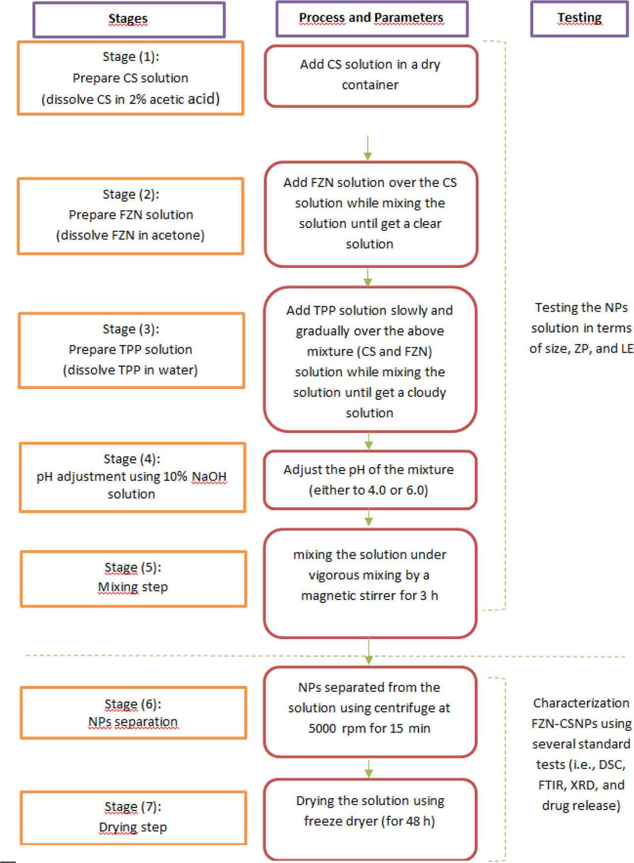
NPs fabrication process flow chart. CS, chitosan; DSC, differential scanning calorimetry; FTIR, Fourier-transform infrared spectroscopy; FZN, fluphenazine; NPs, nanoparticles; TPP, tripolyphosphate; XRD, X-ray diffraction
It is essential to control NPs properties in the fabricating process to indicate and monitor the stability and effectiveness of NPs drug delivery systems. A small NPs size (<200 nm) improves drug permeability and diffusion in the body [36].
On the other hand, ZP is also one of the essential NPs characteristics. ZP indicates the surface electrostatic charge of the NPs. However, a high degree of ZP reflects high resistance to agglomeration, which provides high stability of NPs. The magnitude of ZP (positive or negative) is referred to as the degree of repulsion between particles [37]. ZP values >30 mV indicate good stability and those >60 mV excellent stability. A value of about 20 mV provides only short-term stability; values in the range of −5 mV to +5 mV provide insufficient stability and fast precipitation as a result [38].
LE is another essential characteristic for NPs drug delivery systems. A higher drug LE is desired. LE refers to the percentage of drug that is successfully entrapped into NPs carriers.
NPs size and ZP for the nanocomposite were measured by dynamic light scattering (DLS) technique using Zetasizer Nano (by Malvern, Worcestershire-UK) at Hikma Pharmaceutical Inc. The ultra-centrifuge technique was used to determine FZN drug-free percentage in the prepared nanocomposite. The analysis method was as follows: 5 mL of solution was centrifuged at 5,000 rpm for 30 min, and then the supernatant solution was measured using high-performance liquid chromatography (HPLC) at 260 nm wavelength. Intersil® ODS-3V (5 μm, 4.6 mm × 250 mm) HPLC column was used to analyze the samples. The mobile phase was prepared by mixing 400 mL of methanol, 400 mL acetonitrile, and 200 mL of 0.05 M ammonium acetate. Finally, the mobile phase mixture was filtrated through a 0.45 μm PTFE syringe filter. The column temperature was kept at 25°C temperature, and the flow rate was 2 mL/min.
A calibration curve was constructed by measuring known concentrations of FZN solutions using HPLC and then plotting the peak area vs. the FZN drug amount. However, the FZN drug-free amount was determined using Eq. (1), and then the percentage of drug loaded in nanocomposite (LE%) was calculated using Eq. (2).
In general, a complete mixture of DoE usually provides several points in the design space at each combination level of the mixture with process variables, leading to many experiments; as process variables increase, the design points within the design space increase [39]. Fractional designs are ideal tools to screen several factors at the same time [40]. In this work, as a preliminary study, an extreme vertices (i.e., constrained) mixture-process model with a fractional approach was employed to design the experimental work and screen the interaction effect between the three components (i.e., FZN, CS, and TPP) and the process variables (i.e., mixing time and pH).
An extreme vertices model was implemented because the design space is constrained (FZN level between 5% and 15%, CS level between 22.5% and 72,5%, and TPP level between 22.5% and 72.5%). This screening study was carried out to eliminate any variable that does not statistically influence the responses with different mixture formulations. Accordingly, 16 runs were suggested using fractional design in the mixture-process model by Minitab statistical software. All experiments were tested in terms of size, ZP, and LE.
A complete mixture of DoE is usually provided several points in the design space at each combination level of the mixture with process variables, leading to a high number of experiments; as process variables increase, the design points within the design space increase [41]. Fractional designs are ideal tools to screen several factors at the same time [42]. Thus, a mixture model with a fractional approach was employed to design the experimental work and screen the interaction effect between the three components (i.e., FZN, CS, and TPP) and the process variables (i.e., mixing time and pH) on the three responses (i.e., NPs size, ZP, and LE%). A screening study was carried out to eliminate the effect of any process variable that is not statistically significant on the responses with different mixture formulations. Accordingly, 16 runs were suggested using fractional design in the mixture-process model by Minitab statistical software. All samples were tested in terms of NPs size, ZP, and LE%. According to this screening study, the mixing time factor was proved to be insignificant and hence discarded from the study.
Based on the screening study, a complete mixture-process DoE approach was applied to the significant NPs input fabrication parameters (i.e., FZN, CS, TPP, and pH) to build a design space for the experimental work, followed accordingly by generation of relevant regression models.
In some cases, it is essential to set constraints on the bound of components. This design is called extreme vertices. This design was chosen because the proportions of the three components in the mixture (CS, TPP, and FZN) are interdependent, and the total of the proportions are the same for each experimental run (i.e., the total of the proportions of CS, TPP, and FZN are equal 100%). Also, a process variable was added to the model to be examined in the study (i.e., pH).
In this study, the design was augmented by adding additional points to the study design space, as shown in Figure 3 (augmented design vs. unaugmented design). As a result, 26 combinations were distributed within the design space with four main type points. Type (1) points (coded as •) are located at the vertex (i.e., at the corners of the design space). Type (2) points (coded as ▪) are located at the middle of an edge of the design space. Type (0) point (coded as ♦) is located at the center point of the design space. Type (−1) points (coded as ▴) are distributed at axial points in the simplex design. The region that is within the gray lines represents the study design space according to the predefined constraints. The constraints on components’ mixture were set as follows: FZN (5–15% w/w), CS (22.5–72.5% w/w), and TPP (22.5–72.5% w/w) at two levels of process variable (pH) were 4.0 [coded as (−1)] to 6.0 [coded as (+1)].
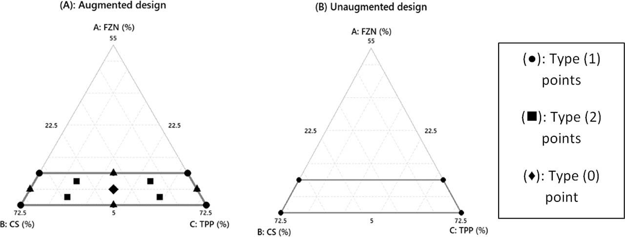
Simples design plot. CS, chitosan; FZN, fluphenazine; TPP, tripolyphosphate
Multivariate regression analysis was carried out on the data collected from the experimental design discussed above, and P-values with a 95% confidence interval (CI) were calculated to determine each model term’s significance using Minitab. The predictors that explain the correlation with the responses were included in the regression model equations accordingly.
Due to the complexity of the models obtained, including some constraints, an optimization-based approach from evolutionary computation was used for finding the optimum NPs fabricating parameters that would meet the predefined objectives (i.e., minimization NPs size, maximization ZP, and maximizing LE%). Eq. (3) illustrates a general constrained MOO [43].
In this study, NSGA-II, as an improved genetic algorithm approach, was used to find the best set of proportions in the mixture with the best process variables involving the fabricating of FZN-CSNPs. The optimum solutions were obtained in the Pareto front as a set of solutions with the best NPs fabrication parameters according to the dominance principle and crowding distance. The non-dominated set solutions were sorted in decreasing order as per crowding distances, and the optimum solutions are having the largest crowding distance values [44].
In general, the NSGA-II algorithm starts creating a random population (P) within the search space with N’s size. Then, the successive generation starts as per predefined iterations. In each iteration, a mating pool is formed to insert solutions from the population P (i.e., parents), and then new individuals Q (i.e., children) are generated using crossover and mutation processes. The new generation is called offspring population (Q) with size (N). However, the combined populations (P + Q) should be ranked according to the non-dominated criterion by creating different fronts (i.e., front 1 to front N) with non-dominated solutions. However, after ranking the solutions from the combined population (P + Q = 2N) in descending order, the crowding distance method is required to select N solutions out of (2N). This method should be applied for maintaining the diversity in the Pareto front [45]. The solutions with higher crowding distance will be selected in descending order (Pt + 1). The cycle will be repeated until the maximum number of generations is achieved, as described in Figure 4. In this study, NSGA-II was coded for three objectives using Python, and it is available for readers upon request.
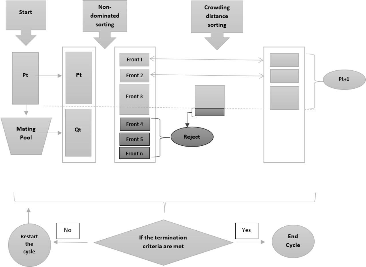
NSGA-II process – adapted from Acampora et al. [46]. NSGA-II, non-dominated sorting genetic algorithm
In this study, the regression models were evaluated in terms of the significance of the independent variables through their reported P-values and the adequacy of the models through their reported coefficient of determination and residuals analysis. Furthermore, tests of hypotheses were carried out to confirm the high level of predictability for the regression models and hence their creditability to serve as objective functions in the optimization step.
Finally, the optimum solution has been fully characterized using different methods such as X-ray diffraction (XRD), Fourier-transform infrared spectroscopy (FTIR), polydispersity index (PdI), differential scanning calorimetry (DSC), and invitro drug release study.
PdI test measures the uniformity of a particle in the solution. PdI value is from (0 −1), where larger PdI values indicate large particle distribution in the sample and agglomeration rate. On the other hand, smaller PdI values indicate small distribution particles with uniform size [47]. PdI test was carried out using Zetasizer (by Malvern) at Hikma Pharmaceutical Inc., Jordan.
DSC is a method used to identify the physical characteristics of NPs powder. DSC measurements were carried out using Mettler Toledo DSC8000, Switzerland (at Hikma Pharmaceutical Inc., Jordan).
In-vitro drug release study was performed using UV-spectrophotometer with λ–max– of 260 nm, in phosphate buffer pH at 7.4 using PerkinElmer UV-Vis. Eq. (4) was used in calculating the drug release percentage.
XRD test is essential to gain an idea of the mixture powder’s crystal structure [48]. The crystal structure of NPs was investigated using XRD at Hikma Pharmaceutical Inc. Diffraction was measured from 2θ (2°–80°) using a Shimadzu X-ray diffractometer, XRD-6000. Three samples were measured: FZN-CSNPs, CSNPs blank, and FZN drug.
FTIR test can be utilized to identify the organic group molecules on the surface of NPs [49]. Any recorded spectrum provides information on a bond’s position and which functional group it is related to, since each functional group has unique absorption characteristics. In this context, the three samples were measured (i.e., FZN-CSNPs, CSNPs blank, and FZN drug) over the range of 400–4,000 cm−1 using PerkinElmer spectrum IR with (4 cm−1) resolution.
Mixture-process model DoE (i.e., extreme vertices) was utilized in this study. The three mixture components [i.e., (A): FZN, (B): CS, and (C): TPP] with the two process variables [i.e., (X1): pH, and (X2): mixing time] were used in experimental design, as shown in Table 1. As discussed earlier, this study was designed to gather data about the predictors and observe the interaction effect between predictors. The screening study facilitates focusing on the significant process variables and carrying out another modeling by designing a complete DoE including augmentations and replications in the design space.
Screening DoE model with experimental values
| Runs | Independent variables | Responses | ||||||
|---|---|---|---|---|---|---|---|---|
| (A) | (B) | (C) | (X1) | (X2) | Size (nm) | ZP (mV) | LE (%) | |
| Run 1 | 15 | 62.5 | 22.5 | 6.0 | 18 | 252 | 7.9 | 97.6 |
| Run 2 | 15 | 22.5 | 62.5 | 6.0 | 3 | 219 | 4.0 | 96.8 |
| Run 3 | 5 | 22.5 | 72.5 | 6.0 | 18 | 324 | 4.4 | 94.0 |
| Run 4 | 5 | 72.5 | 22.5 | 4.0 | 3 | 152 | 24.0 | 85.8 |
| Run 5 | 15 | 62.5 | 22.5 | 6.0 | 3 | 258 | 8.0 | 97.4 |
| Run 6 | 5 | 22.5 | 72.5 | 6.0 | 3 | 389 | 4.3 | 94.2 |
| Run 7 | 15 | 22.5 | 62.5 | 6.0 | 18 | 197 | 4.5 | 97.0 |
| Run 8 | 5 | 72.5 | 22.5 | 6.0 | 3 | 279 | 7.2 | 92.6 |
| Run 9 | 15 | 62.5 | 22.5 | 4.0 | 3 | 148 | 24.1 | 91.2 |
| Run 10 | 15 | 62.5 | 22.5 | 4.0 | 18 | 159 | 21.2 | 91.1 |
| Run 11 | 5 | 22.5 | 72.5 | 4.0 | 18 | 549 | 6.9 | 83.4 |
| Run 12 | 15 | 22.5 | 62.5 | 4.0 | 3 | 642 | 7.6 | 84.6 |
| Run 13 | 5 | 72.5 | 22.5 | 4.0 | 18 | 150 | 28.0 | 84.0 |
| Run 14 | 5 | 72.5 | 22.5 | 6.0 | 18 | 279 | 7.9 | 92.7 |
| Run 15 | 5 | 22.5 | 72.5 | 4.0 | 3 | 302 | 6.8 | 83.3 |
| Run 16 | 15 | 22.5 | 62.5 | 4.0 | 18 | 631 | 7.6 | 84.8 |
Note: (A): FZN%, (B): CS%, (C): TPP%, (X1): pH, and (X2): mixing time.
CS, chitosan; FZN, fluphenazine; LE, loading efficiency; TPP, tripolyphosphate; ZP, zeta potential.
ANOVA using mixture regression was carried out on the three responses’ data (i.e., size, ZP, and LE). Results indicated that there were significant interaction effects between the pH variable (X1) and the three mixture components (A, B, and C) based on the P-values obtained (i.e., <0.05), as shown in the analysis of the three responses (refer to Tables 2–4). Although there were some non-significant interaction effects revealed between the components of the mixture and pH value (such as AX1, CX1, and ABX1) in ZP analysis, there was another important interaction effect detected in ZP analysis (like in BX1), as shown in Table 3. On the other hand, there is no significant interaction effect or main effect indicated between any of the mixture components (A, B, and C) and mixing time variable (X2) at both levels (high and low levels) on any of the three responses based on the P-values for the interaction, which are higher than the significance level (i.e., 0.05), as shown in Tables 2–4. Thus, the effect of mixing time is not statistically significant. Tables 2–4 do not display the P-values for the main effect for the mixture components because all components are dependent on each other. For process variables, no statistical evidence is available to support the view that the main significant effect (i.e., linear effect) for mixing time process variable affects the three responses according to the P-values. On the other hand, there is statistical evidence that the main significant effect (i.e., linear effect) for pH process variable affects the three responses according to the P-values.
ANOVA for size-screening study
| Source | DF | Seq SS | Adj SS | Adj MS | F-value | P-value |
|---|---|---|---|---|---|---|
| Regression | 11 | 65411864 | 65411864 | 5946533 | 901.35 | 0.000 |
| Component only | ||||||
| Linear | 2 | 16852012 | 25941727 | 12970863 | 1966.06 | 0.000 |
| Quadratic | 1 | 10563934 | 10563934 | 10563934 | 1601.23 | 0.000 |
| A × B | 1 | 10563934 | 10563934 | 10563934 | 1601.23 | 0.000 |
| Component × X1 | ||||||
| Linear | 3 | 26622324 | 34654360 | 11551453 | 1750.92 | 0.000 |
| A × X1 | 1 | 16413096 | 19779395 | 19779395 | 2998.07 | 0.000 |
| B × X1 | 1 | 9152068 | 955902 | 955902 | 144.89 | 0.000 |
| C × X1 | 1 | 1057159 | 3609045 | 3609045 | 547.04 | 0.000 |
| Quadratic | 1 | 11360884 | 11360884 | 11360884 | 1722.03 | 0.000 |
| A × B × X1 | 1 | 11360884 | 11360884 | 11360884 | 1722.03 | 0.000 |
| Component × X2 | ||||||
| Linear | 3 | 6511 | 12619 | 4206 | 0.64 | 0.629 |
| A × X2 | 1 | 520 | 10879 | 10879 | 1.65 | 0.268 |
| B × X2 | 1 | 1446 | 1701 | 1701 | 0.26 | 0.638 |
| C × X2 | 1 | 4545 | 10744 | 10744 | 1.63 | 0.271 |
| Quadratic | 1 | 6200 | 6200 | 6200 | 0.94 | 0.387 |
| A × B × X2 | 1 | 6200 | 6200 | 6200 | 0.94 | 0.387 |
| Residual Error | 4 | 26390 | 26390 | 6597 | ||
| Total | 15 | 65438254 |
Note: (A): FZN%, (B): CS%, (C): TPP%, (X1): pH, and (X2): mixing time.
ANOVA, analysis of variance; CS, chitosan; FZN, fluphenazine; TPP, tripolyphosphate.
ANOVA for ZP-screening study
| Source | DF | Seq SS | Adj SS | Adj MS | F-value | P-value |
|---|---|---|---|---|---|---|
| Regression | 11 | 1008.68 | 1008.68 | 91.698 | 77.30 | 0.000 |
| Component only | ||||||
| Linear | 2 | 426.63 | 256.25 | 128.124 | 108.01 | 0.000 |
| Quadratic | 1 | 0.23 | 0.23 | 0.231 | 0.19 | 0.682 |
| A × B | 1 | 0.23 | 0.23 | 0.231 | 0.19 | 0.682 |
| Component × X1 | ||||||
| Linear | 3 | 573.36 | 152.82 | 50.940 | 42.94 | 0.002 |
| A × X1 | 1 | 282.00 | 0.29 | 0.288 | 0.24 | 0.648 |
| B × X1 | 1 | 284.68 | 109.49 | 109.488 | 92.30 | 0.001 |
| C × X1 | 1 | 6.68 | 5.15 | 5.147 | 4.34 | 0.106 |
| Quadratic | 1 | 0.61 | 0.61 | 0.606 | 0.51 | 0.514 |
| A × B × X1 | 1 | 0.61 | 0.61 | 0.606 | 0.51 | 0.514 |
| Component × X2 | ||||||
| Linear | 3 | 4.00 | 7.66 | 2.553 | 2.15 | 0.236 |
| A × X2 | 1 | 0.08 | 0.91 | 0.914 | 0.77 | 0.430 |
| B × X2 | 1 | 2.84 | 6.67 | 6.671 | 5.62 | 0.077 |
| C × X2 | 1 | 1.08 | 0.67 | 0.671 | 0.57 | 0.494 |
| Quadratic | 1 | 3.84 | 3.84 | 3.842 | 3.24 | 0.146 |
| A × B × X2 | 1 | 3.84 | 3.84 | 3.842 | 3.24 | 0.146 |
| Residual Error | 4 | 4.74 | 4.74 | 1.186 | ||
| Total | 15 | 1013.42 |
Note: (A): FZN%, (B): CS%, (C): TPP%, (X1): pH, and (X2): mixing time.
ANOVA, analysis of variance; CS, chitosan; FZN, fluphenazine; TPP, tripolyphosphate; ZP, zeta potential.
ANOVA for LE-screening study
| Source | DF | Seq SS | Adj SS | Adj MS | F-value | P-value |
|---|---|---|---|---|---|---|
| Regression | 11 | 448.552 | 448.552 | 40.7774 | 172.15 | 0.000 |
| Component Only | ||||||
| Linear | 2 | 68.186 | 10.791 | 5.3954 | 22.78 | 0.007 |
| Quadratic | 1 | 14.811 | 14.811 | 14.8113 | 62.53 | 0.001 |
| A × B | 1 | 14.811 | 14.811 | 14.8113 | 62.53 | 0.001 |
| Component × X1 | ||||||
| Linear | 3 | 361.159 | 190.177 | 63.3923 | 267.62 | 0.000 |
| A × X1 | 1 | 274.911 | 4.726 | 4.7263 | 19.95 | 0.011 |
| B × X1 | 1 | 7.779 | 10.489 | 10.4893 | 44.28 | 0.003 |
| C × X1 | 1 | 78.468 | 18.425 | 18.4246 | 77.78 | 0.001 |
| Quadratic | 1 | 3.629 | 3.629 | 3.6288 | 15.32 | 0.017 |
| A × B × X1 | 1 | 3.629 | 3.629 | 3.6288 | 15.32 | 0.017 |
| Component × X2 | ||||||
| Linear | 3 | 0.694 | 0.733 | 0.2442 | 1.03 | 0.469 |
| A × X2 | 1 | 0.001 | 0.000 | 0.0000 | 0.00 | 0.995 |
| B × X2 | 1 | 0.681 | 0.493 | 0.4929 | 2.08 | 0.223 |
| C × X2 | 1 | 0.013 | 0.018 | 0.0177 | 0.07 | 0.798 |
| Quadratic | 1 | 0.073 | 0.073 | 0.0732 | 0.31 | 0.608 |
| A × B × X2 | 1 | 0.073 | 0.073 | 0.0732 | 0.31 | 0.608 |
| Residual Error | 4 | 0.948 | 0.948 | 0.2369 | ||
| Total | 15 | 449.499 |
Note: (A): FZN%, (B): CS%, (C): TPP%, (X1): pH, and (X2): mixing time.
ANOVA, analysis of variance; CS, chitosan; FZN, fluphenazine; LE, loading efficiency; TPP, tripolyphosphate.
Accordingly, mixing time was not considered for further investigation as a variable in the complete mixture DoE. Hence, mixing time will be adjusted at a lower level (i.e., 3 h), because this will accelerate the fabrication process, in turn resulting in greater efficiency in the production of NPs in controlled morphology and distribution [50]. On the other hand, the following parameters, FZN%, CS%, TPP%, and pH value, will be considered as NPs input fabrication parameters for further investigation.
A complete randomized design was employed to design the experimental model. Also, three replications were considered to reduce the experimental error.
Table 5 summarizes the three responses’ data (i.e., NPs size, ZP, and LE%) for the 26 combinations (i.e., F01-F26, three replicates for each combination) suggested by the mixture design, and the corresponding experimental procedures were carried out in the laboratory.
Complete DoE study-data
| Run codes | Non-dependent variables | Responses | |||||
|---|---|---|---|---|---|---|---|
| (FZN) | (CS) | (TPP) | (pH) | Size | ZP | LE | |
| F01-1 | 5.0 | 72.50 | 22.50 | 6.0 | 225 | 7 | 82 |
| F01-2 | 5.0 | 72.50 | 22.50 | 6.0 | 221 | 7 | 81 |
| F01-3 | 5.0 | 72.50 | 22.50 | 6.0 | 221 | 8 | 81 |
| F02-1 | 12.5 | 53.75 | 33.75 | 4.0 | 253 | 14 | 80 |
| F02-2 | 12.5 | 53.75 | 33.75 | 4.0 | 262 | 16 | 80 |
| F02-3 | 12.5 | 53.75 | 33.75 | 4.0 | 257 | 16 | 79 |
| F03-1 | 10.0 | 45.00 | 45.00 | 6.0 | 255 | 5 | 87 |
| F03-2 | 10.0 | 45.00 | 45.00 | 6.0 | 262 | 5 | 90 |
| F03-3 | 10.0 | 45.00 | 45.00 | 6.0 | 259 | 6 | 90 |
| F04-1 | 15.0 | 42.50 | 42.50 | 4.0 | 626 | 12 | 83 |
| F04-2 | 15.0 | 42.50 | 42.50 | 4.0 | 625 | 10 | 82 |
| F04-3 | 15.0 | 42.50 | 42.50 | 4.0 | 627 | 12 | 82 |
| F05-1 | 7.5 | 33.75 | 58.75 | 4.0 | 687 | 7 | 80 |
| F05-2 | 7.5 | 33.75 | 58.75 | 4.0 | 686 | 9 | 81 |
| F05-3 | 7.5 | 33.75 | 58.75 | 4.0 | 670 | 9 | 79 |
| F06-1 | 5.0 | 47.50 | 47.50 | 6.0 | 209 | 5 | 84 |
| F06-2 | 5.0 | 47.50 | 47.50 | 6.0 | 203 | 5 | 88 |
| F06-3 | 5.0 | 47.50 | 47.50 | 6.0 | 217 | 5 | 83 |
| F07-1 | 15.0 | 22.50 | 62.50 | 4.0 | 499 | 9 | 70 |
| F07-2 | 15.0 | 22.50 | 62.50 | 4.0 | 514 | 7 | 70 |
| F07-3 | 15.0 | 22.50 | 62.50 | 4.0 | 502 | 9 | 69 |
| F08-1 | 7.5 | 33.75 | 58.75 | 6.0 | 297 | 4 | 88 |
| F08-2 | 7.5 | 33.75 | 58.75 | 6.0 | 307 | 4 | 87 |
| F08-3 | 7.5 | 33.75 | 58.75 | 6.0 | 317 | 4 | 87 |
| F09-1 | 10.0 | 45.00 | 45.00 | 4.0 | 501 | 16 | 82 |
| F09-2 | 10.0 | 45.00 | 45.00 | 4.0 | 506 | 16 | 83 |
| F09-3 | 10.0 | 45.00 | 45.00 | 4.0 | 504 | 16 | 81 |
| F10-1 | 7.5 | 58.75 | 33.75 | 6.0 | 164 | 6 | 87 |
| F10-2 | 7.5 | 58.75 | 33.75 | 6.0 | 179 | 6 | 86 |
| F10-3 | 7.5 | 58.75 | 33.75 | 6.0 | 164 | 6 | 86 |
| F11-1 | 12.5 | 53.75 | 33.75 | 6.0 | 299 | 6 | 91 |
| F11-2 | 12.5 | 53.75 | 33.75 | 6.0 | 296 | 6 | 91 |
| F11-3 | 12.5 | 53.75 | 33.75 | 6.0 | 297 | 6 | 91 |
| F12-1 | 15.0 | 62.50 | 22.50 | 6.0 | 228 | 8 | 91 |
| F12-2 | 15.0 | 62.50 | 22.50 | 6.0 | 221 | 8 | 91 |
| F12-3 | 15.0 | 62.50 | 22.50 | 6.0 | 230 | 8 | 92 |
| F13-1 | 5.0 | 22.50 | 72.50 | 6.0 | 276 | 4 | 84 |
| F13-2 | 5.0 | 22.50 | 72.50 | 6.0 | 264 | 4 | 84 |
| F13-3 | 5.0 | 22.50 | 72.50 | 6.0 | 272 | 4 | 84 |
| F14-1 | 12.5 | 33.75 | 53.75 | 6.0 | 226 | 5 | 91 |
| F14-2 | 12.5 | 33.75 | 53.75 | 6.0 | 225 | 5 | 91 |
| F14-3 | 12.5 | 33.75 | 53.75 | 6.0 | 225 | 6 | 91 |
| F15-1 | 7.5 | 58.75 | 33.75 | 4.0 | 360 | 16 | 74 |
| F15-2 | 7.5 | 58.75 | 33.75 | 4.0 | 360 | 16 | 74 |
| F15-3 | 7.5 | 58.75 | 33.75 | 4.0 | 360 | 19 | 74 |
| F16-1 | 10.0 | 22.50 | 67.50 | 6.0 | 277 | 4 | 89 |
| F16-2 | 10.0 | 22.50 | 67.50 | 6.0 | 265 | 5 | 90 |
| F16-3 | 10.0 | 22.50 | 67.50 | 6.0 | 267 | 4 | 90 |
| F17-1 | 10.0 | 67.50 | 22.50 | 4.0 | 195 | 20 | 88 |
| F17-2 | 10.0 | 67.50 | 22.50 | 4.0 | 190 | 22 | 88 |
| F17-3 | 10.0 | 67.50 | 22.50 | 4.0 | 191 | 23 | 88 |
| F18-1 | 5.0 | 72.50 | 22.50 | 4.0 | 167 | 16 | 82 |
| F18-2 | 5.0 | 72.50 | 22.50 | 4.0 | 168 | 22 | 82 |
| F18-3 | 5.0 | 72.50 | 22.50 | 4.0 | 164 | 22 | 82 |
| F19-1 | 10.0 | 22.50 | 67.50 | 4.0 | 353 | 7 | 83 |
| F19-2 | 10.0 | 22.50 | 67.50 | 4.0 | 351 | 7 | 83 |
| F19-3 | 10.0 | 22.50 | 67.50 | 4.0 | 351 | 7 | 83 |
| F20-1 | 5.0 | 22.50 | 72.50 | 4.0 | 428 | 7 | 79 |
| F20-2 | 5.0 | 22.50 | 72.50 | 4.0 | 433 | 8 | 79 |
| F20-3 | 5.0 | 22.50 | 72.50 | 4.0 | 427 | 7 | 79 |
| F21-1 | 15.0 | 22.50 | 62.50 | 6.0 | 458 | 5 | 96 |
| F21-2 | 15.0 | 22.50 | 62.50 | 6.0 | 438 | 5 | 96 |
| F21-3 | 15.0 | 22.50 | 62.50 | 6.0 | 447 | 5 | 96 |
| F22-1 | 5.0 | 47.50 | 47.50 | 4.0 | 414 | 11 | 80 |
| F22-2 | 5.0 | 47.50 | 47.50 | 4.0 | 404 | 12 | 80 |
| F22-3 | 5.0 | 47.50 | 47.50 | 4.0 | 424 | 16 | 80 |
| F23-1 | 10.0 | 67.50 | 22.50 | 6.0 | 239 | 7 | 89 |
| F23-2 | 10.0 | 67.50 | 22.50 | 6.0 | 237 | 7 | 89 |
| F23-3 | 10.0 | 67.50 | 22.50 | 6.0 | 240 | 8 | 89 |
| F24-1 | 15.0 | 62.50 | 22.50 | 4.0 | 185 | 18 | 91 |
| F24-2 | 15.0 | 62.50 | 22.50 | 4.0 | 181 | 20 | 91 |
| F24-3 | 15.0 | 62.50 | 22.50 | 4.0 | 183 | 20 | 91 |
| F25-1 | 12.5 | 33.75 | 53.75 | 4.0 | 528 | 10 | 82 |
| F25-2 | 12.5 | 33.75 | 53.75 | 4.0 | 511 | 12 | 82 |
| F25-3 | 12.5 | 33.75 | 53.75 | 4.0 | 507 | 14 | 82 |
| F26-1 | 15.0 | 42.50 | 42.50 | 6.0 | 232 | 6 | 92 |
| F26-2 | 15.0 | 42.50 | 42.50 | 6.0 | 230 | 6 | 92 |
| F26-3 | 15.0 | 42.50 | 42.50 | 6.0 | 230 | 6 | 92 |
Note: Run codes can be read as follows: F (Run number-replicate number). For example, F03-2 means the 2nd replicate in the 3rd run.
CS, chitosan; FZN, fluphenazine; LE, loading efficiency; TPP, tripolyphosphate; ZP, zeta potential.
ANOVA indicates that all NPs input fabrication parameters are statistically significant. Besides, the predictors’ interactions showed high statistical significance (P-values are less than the significance level of 0.05). Three regression models have been generated accordingly. Eqs (5)–(7) represent the regression equations for the three objectives generated after performing mixture regression analysis using Minitab.
The main effect plots are considered a visualization method to examine how the pH influences the responses to the question of whether the variables interact. Figure 5 indicates that the pH significantly affects the three responses with differing patterns because the main effect line is not drawn horizontally in any of the predictors. As pH increases, NPs size and ZP decrease, as indicated in Figure 5A, 5B. In contrast, LE% increases as the pH value increases, as indicated in Figure 5C.
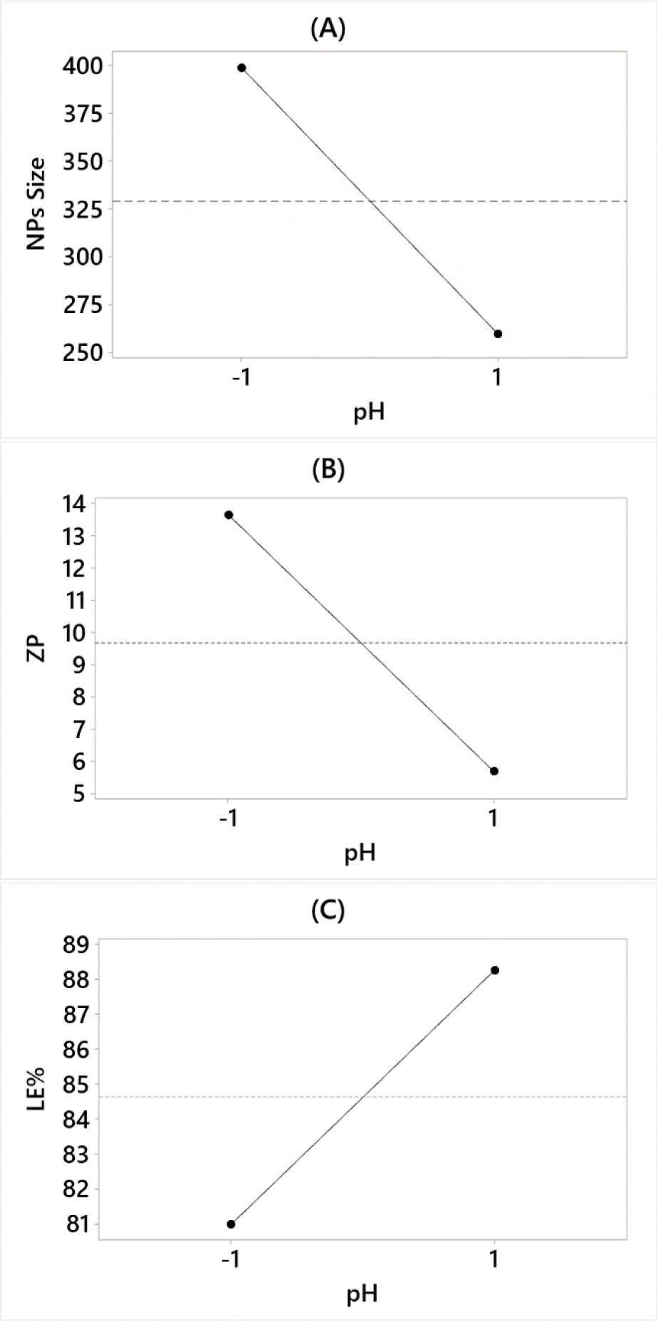
Main effect plots. LE, loading efficiency; NPs, nanoparticles
Figure 6A–6C shows the contour plots for the three responses. The plots at the left side represent the mixture formulation when prepared at the low pH level (i.e., pH = 4.0), whereas the plots at the right side represent the high level of pH (i.e., pH = 6.0). The region that is within the solid gray lines represents the design space of the study.
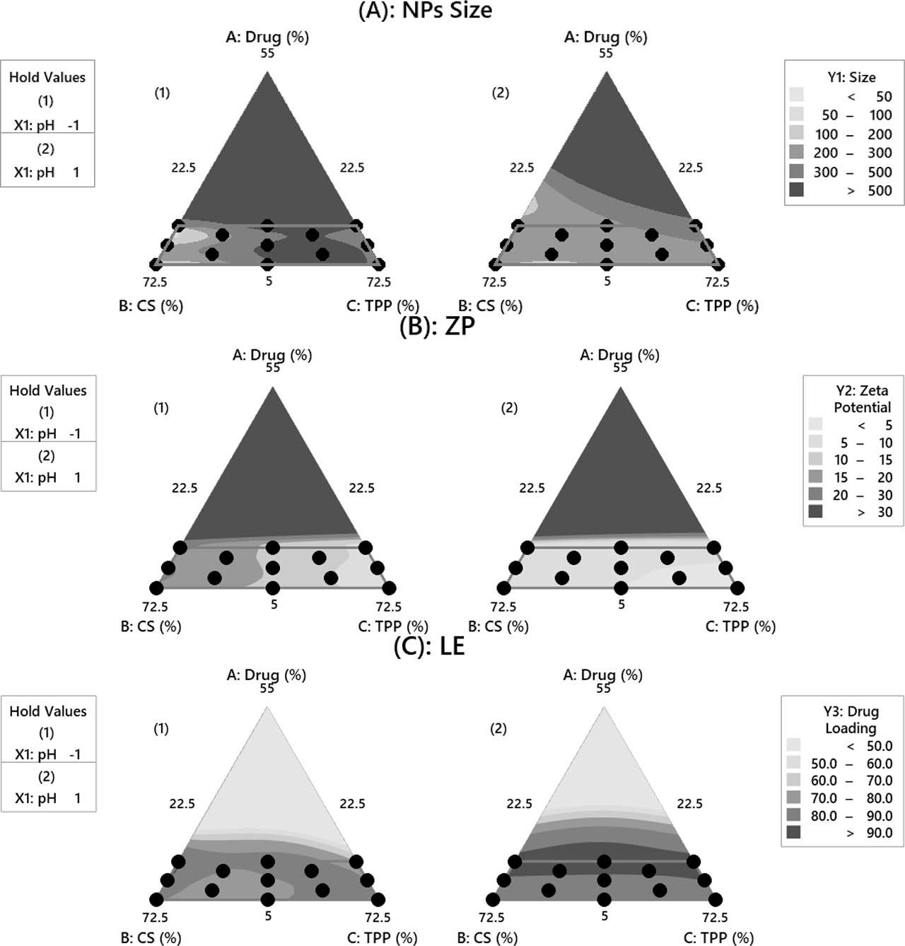
Contour plots. CS, chitosan; LE, loading efficiency; NPs, nanoparticles; TPP, tripolyphosphate; ZP, zeta potential
Figure 6A represents the contour plots for size and illustrates how proportions of the component’s mixture affect the size of NPs. If the mixture’s component proportions are chosen from the lower-left corner of the study design space, NPs size would be the smallest. On the other hand, NPs size would increase if the mixture’s component proportions are chosen from the design space’s right corner (regardless of the solution’s pH). In both plots (right and left), the light gray area represents the best for size. Since the NPs size would be reduced at a low pH level, the effect of the process variable (i.e., pH of solution) on size is perceptible in the case of both plots. The left corner area represents the best blend of the components within the constrained design space. Preparing FZN-CSNPs nanocomposite with reference to the design space study region and using the following NPs input fabrication parameters, i.e., FZN = 15%, CS = 62.5%, TPP = 22.5%, and pH = 4.0, similar to the F24 parameters shown in Table 1, would produce NPs with small sizes.
Figure 6B represents the contour plots for ZP. The light gray area represents the worst for ZP (lowest values). On the other hand, the dark gray area (at the lower-left corner) represents the best for ZP (highest values), especially at a lower pH level. Preparing FZN-CSNPs nanocomposite with reference to the design space study region and using the following NPs input fabrication parameters, i.e., FZN = 15%, CS = 62.5%, TPP = 22.5%, and pH = 4.0, similar to the F24 parameters shown in Table 1, would produce NPs with best ZP values. The contour plots for LE are demonstrated in Figure 6C. The light gray areas in the entire design space represent the lowest LE values (especially at the upper corner). In comparison, the dark gray area represents the best for LE (highest values) that are located at the middle borderline. Preparing FZN-CSNPs nanocomposite with reference to the design space study region and using the following NPs input fabrication parameters, i.e., FZN = 15%, CS = 22.5%, TPP = 62.5%, and pH = 6.0, similar to the F24 parameters shown in Table 1, would produce NPs with best LE values.
In summary, one mixture with a high percentage of CS, low percentage of TPP, and low pH value is required to achieve the first two objectives (NPs size maximization and ZP minimization). In contrast, a mixture with a low percentage of CS, a high percentage of TPP, and high pH is required to achieve the third objective (LE maximization). Nevertheless, in all cases, a high percentage of FZN is required to achieve the three objectives. Thus, there was a need for the use of NSGA-II to deal with these conflicting objectives.
Table 6 summarizes the values of R-seq, adjusted R-seq, and predicted R-seq for the three objectives. In this study, high values of [R-seq and adjusted R-seq] represent how the model fits data and how much of the responses’ variation is explained by the predictors inserted in each model. Additionally, high values of R-seq predicted (94.12%, 93.79%, and 91.61%) show how well the model predicts the three responses (i.e., NPs size, ZP, and LE%, respectively) for new observations according to Eqs (5)–(7).
Regression model evaluations
| Model | R-seq (%) | R-seq (adj) (%) | R-seq (pred) (%) |
|---|---|---|---|
| Model (1): size | 96.23 | 95.24 | 94.12 |
| Model (2): ZP | 96.05 | 95.09 | 93.79 |
| Model (3): IE | 94.44 | 92.98 | 91.61 |
ZP, zeta potential.
Analysis of residuals is one approach to verify the model’s goodness [51]. Some assumptions should be evaluated before using the model to predict the concerned objective [52]. The first assumption that the residuals should be normally distributed. Figure 7 represents residual analysis in multiple plots (i.e., normal probability plot, residuals vs. observation order plot, residuals vs. fitted value plot, and histogram plot). In this study, the normal probability plots indicate that all residuals approximately follow a straight line in a linear pattern. Thus, the normality assumption was met.
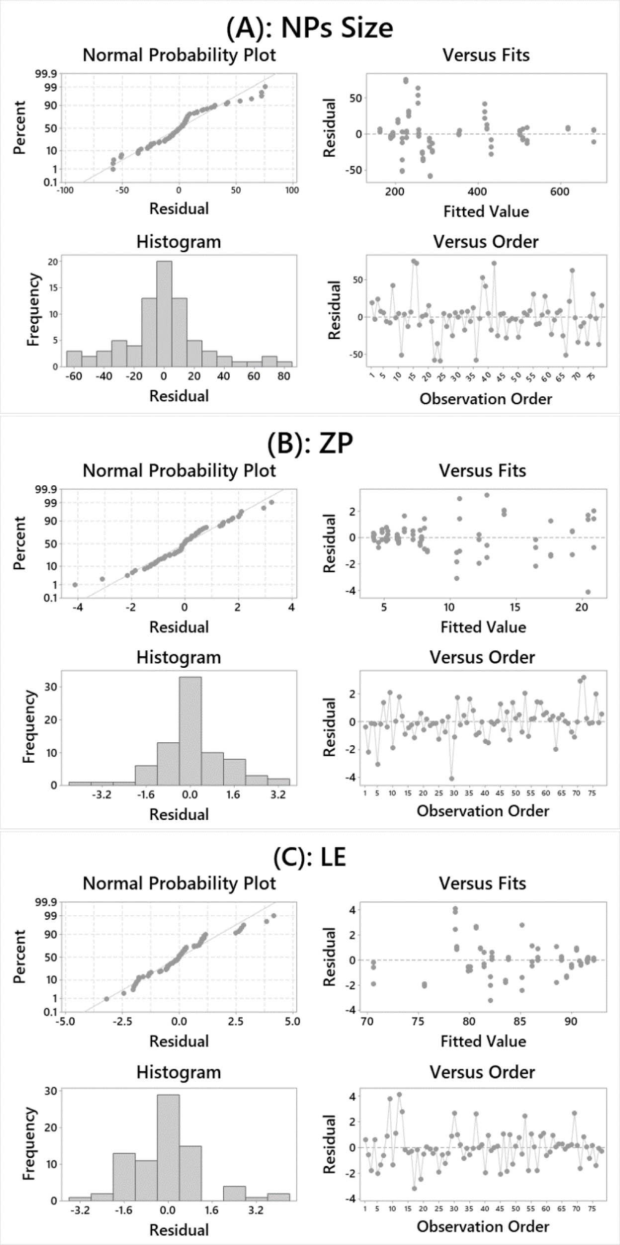
Analysis of residuals. LE, loading efficiency; NPs, nanoparticles; ZP, zeta potential
The second assumption is that independence in the observations should be met during residual analysis. The residuals vs. observation order plots in Figure 7 indicate that there are no trends observed in time order, and that all residuals fall randomly around the centerline on the plots for all responses. Residuals vs. fitted value plot is a visualized method to verify the third assumption that the residual should be randomly distributed with constant variance [53]. In this study, the residuals vs. fitted value plots show that all residuals points fall randomly above and under zero line with no trends or patterns observed. Histogram plots are constructed for residuals to enable their distribution to be displayed and verify if there any outliers [54]. In this study, histogram plots show that the residuals for all observations generated from the three responses were approximately skewed with one long bar. Besides, there are bars distributed away from other bars. Thus, no outliers are detected.
When NPs are fabricated using the different techniques, the resultant size is usually within a range of 100–300 nm [55]. ZP is also an essential objective to ensure the stability of NPs. High ZP causes larger repulsive forces between particles, and this prevents aggregation of the NPs. However, in some cases, NPs with a ZP of 20 mV or much lower are acceptable and can provide some stabilization [38]. A perusal of the literature indicates that, within nanocomposite application, all Pareto front solutions are acceptable in terms of LE%. For instance, gemcitabine NPs yielded a drug loading range of 70–83% [56].
Table 7 represents a set of 66 Pareto optimal solutions that were provided as superior solutions from the global design space. The Pareto front offered a diverse NPs size within a range of 126.6–238.9 nm, but smaller is favorable. In contrast, a wide range is provided for ZP data (4.9–21.5 mV), but at the very minimum, it is expected that ZP should be >18 mV; NPs with a ZP of 20 mV or much lower are acceptable and can provide some stabilization [38]. Lastly, all LE% data are within a tight range of 88.8–91.2%; therefore, any solution provided in the Pareto front is satisfactory in terms of LE%. Consequently, choosing one solution as the trade-off points should be primarily based on the first objective (i.e., size). However, trade-off points is an approach to compromise between the objective function and the decision-maker [30]. The solution of S19 was chosen to be the trade-off points. This solution has predicted values of 126.6 nm, 18.7 mV, and 91.6% for size, ZP, and LE%, respectively. Thus, the optimum formulation parameters to achieve the optimal objectives (i.e., S19) are 13.3% of FZN, 64.2% of CS, 22.5% TPP, and pH at 4.0.
Pareto solutions
| Solution no. | Size | ZP | LE |
|---|---|---|---|
| S1 | 215.6 | 21.5 | 88.8 |
| S2 | 204.1 | 21.4 | 89.4 |
| S3 | 198.0 | 21.3 | 89.6 |
| S4 | 191.9 | 21.2 | 89.8 |
| S5 | 183.2 | 20.8 | 89.5 |
| S6 | 171.2 | 20.7 | 90.4 |
| S7 | 167.2 | 20.6 | 90.7 |
| S8 | 165.3 | 20.5 | 90.6 |
| S9 | 153.0 | 20.2 | 91.1 |
| S10 | 147.9 | 20.0 | 91.2 |
| S11 | 145.5 | 19.9 | 91.3 |
| S12 | 143.2 | 19.8 | 91.3 |
| S13 | 141.0 | 19.7 | 91.4 |
| S14 | 138.4 | 19.5 | 91.3 |
| S15 | 136.5 | 19.2 | 91.1 |
| S16 | 132.7 | 19.0 | 91.2 |
| S17 | 129.4 | 18.9 | 91.4 |
| S18 | 127.2 | 18.8 | 91.6 |
| S19 | 126.6 | 18.7 | 91.6 |
| S20 | 164.6 | 4.9 | 91.7 |
| S21 | 164.6 | 4.9 | 91.7 |
| S22 | 165.1 | 5.0 | 91.7 |
| S23 | 168.9 | 5.1 | 91.7 |
| S24 | 177.1 | 5.2 | 91.7 |
| S25 | 173.6 | 4.9 | 91.8 |
| S26 | 177.9 | 5.1 | 91.8 |
| S27 | 177.2 | 5.0 | 91.9 |
| S28 | 177.2 | 5.0 | 91.9 |
| S29 | 184.3 | 5.2 | 91.8 |
| S30 | 186.1 | 5.3 | 91.8 |
| S31 | 190.7 | 5.4 | 91.7 |
| S32 | 181.4 | 5.1 | 91.9 |
| S33 | 189.1 | 5.3 | 91.9 |
| S34 | 192.7 | 5.4 | 91.8 |
| S35 | 195.5 | 5.5 | 91.8 |
| S36 | 199.9 | 5.6 | 91.7 |
| S37 | 189.8 | 5.1 | 92.0 |
| S38 | 194.2 | 5.4 | 91.9 |
| S39 | 200.4 | 5.6 | 91.8 |
| S40 | 194.4 | 5.2 | 92.0 |
| S41 | 194.5 | 5.3 | 92.0 |
| S42 | 200.7 | 5.6 | 91.9 |
| S43 | 203.7 | 5.7 | 91.8 |
| S44 | 201.8 | 5.2 | 92.1 |
| S45 | 205.4 | 5.7 | 91.9 |
| S46 | 214.8 | 6.0 | 91.7 |
| S47 | 207.3 | 5.3 | 92.1 |
| S48 | 205.6 | 5.6 | 92.0 |
| S49 | 208.8 | 5.8 | 91.9 |
| S50 | 211.3 | 5.5 | 92.1 |
| S51 | 216.9 | 6.0 | 91.9 |
| S52 | 217.2 | 6.1 | 91.9 |
| S53 | 220.8 | 6.2 | 91.8 |
| S54 | 221.9 | 5.5 | 92.2 |
| S55 | 217.0 | 5.9 | 92.0 |
| S56 | 217.8 | 6.0 | 92.0 |
| S57 | 221.5 | 6.2 | 91.9 |
| S58 | 223.7 | 6.3 | 91.8 |
| S59 | 225.9 | 6.4 | 91.8 |
| S60 | 230.7 | 6.5 | 91.7 |
| S61 | 223.2 | 6.0 | 92.1 |
| S62 | 223.6 | 6.1 | 92.0 |
| S63 | 227.2 | 6.4 | 91.9 |
| S64 | 231.8 | 6.6 | 91.8 |
| S65 | 234.8 | 6.7 | 91.8 |
| S66 | 238.9 | 6.8 | 91.7 |
LE, loading efficiency; ZP, zeta potential.
NSGA-II algorithm has been coded in Python platform. However, to eliminate the possibility of the search process being a primitive random search, the mutation rate parameter should be kept low, typically in a range of 0.1–0.2% [57]. A total of 1,400–1,800 iterations should be carried out to generate satisfactory data [57]. In this study, NSGAII algorithm parameters were identified as follows: population size of 5,000, generation size of 1,500, mutation rate of 0.2, and crossover rate of 0.3. In this study, the three objectives’ fitness functions were constructed based on the regression models and predefined constraints shown in Eqs (5)–(7).
The mathematical models obtained from the regression analysis [i.e., Eqs (5)–(7)] were validated to ensure that they were sufficiently reliable for prediction purposes. Accordingly, the optimized NPs input fabrication parameters (i.e., the tradeoff points) suggested by Pareto front were prepared in the lab in nine replicates, and the samples were tested in terms of NPs size, ZP, and LE%. Table 8 indicates that the nine replications’ observed results were satisfactory, matching with the predicted values of 126.6 nm, 18.8 mV, and 91.6%, respectively.
Validation experiments – data
| Run codes | NPs input fabrication parameters | Size (nm) | ZP (mV) | LE (%) | ||||||
|---|---|---|---|---|---|---|---|---|---|---|
| A | B | C | X−1 | Experimental Values | Predicted using Eq. (5) | Experimental | Predicted using Eq. (6) | Experimental Values | Predicted using Eq. (7) | |
| V1 | 131.0 | 20.4 | 93.0 | |||||||
| V2 | 130.0 | 21.3 | 91.3 | |||||||
| V3 | 128.2 | 20.0 | 92.6 | |||||||
| V4 | 13.3% | 64.2% | 22.5% | 4.0 | 125.4 | 126.6 | 19.0 | 18.7 | 91.4 | 91.6% |
| V5 | 129.0 | 22.0 | 92.0 | |||||||
| V6 | 132.0 | 20.0 | 93.1 | |||||||
| V7 | 125.4 | 17.7 | 92.5 | |||||||
| V8 | 126.0 | 18.0 | 90.4 | |||||||
| V9 | 127.0 | 18.4 | 92.5 | |||||||
| Mean | 128.2 | 126.6 | 19.6 | 18.7 | 92.1 | 91.6 | ||||
| Standard Deviation | 2.45 | – | 1.48 | – | 0.90 | – | ||||
| Test of hypothesis | H0: μ = 126.6 | H0: μ =18.7 | H0: μ = 91.6 | |||||||
| H1: μ ≠ 126.6 | H1: μ ≠ 18.7 | H1: μ ≠ 91.6 | ||||||||
| P-value | P-value = 0.082 | P-value = 0.092 | P-value = 0.140 | |||||||
| 95% CI for μ | (126.3–130.1 nm) | (18.5 – 20.8 mV) | (91.4–92.8%) | |||||||
CI, confidence interval; LE, loading efficiency; NPs, nanoparticles; ZP, zeta potential.
Hypothesis testing of a single mean approach (predicted vs. observed) was utilized to ensure that the models predict the responses accurately and precisely. One-sample t-test was performed using Minitab to determine whether there was any statistically significant difference between the population mean (i.e., the mean of observed data “μ”) and the reference value (i.e., the predicted value “μ–0–”). The P-value should be compared to the significant level (i.e., 0.05). The null hypothesis states that the observed samples’ mean is equal to the hypothesized mean value (μ– = –μ–0–). In contrast, the two means are not equal, as stated in the alternative hypothesis (μ– ≠ –μ–0–). Results show that the P-values for all responses (size, ZP, and LE%) are higher than the significance level (0.082, 0.092, and 0.140, respectively), which means there is a failure to reject the null hypothesis; this allows us to conclude that the observed data’s means are not significantly different from the target values (i.e., predicted values). Furthermore, the standard deviations (StDev.) for the three data groups are relatively low (i.e., 2.45, 1.48, and 0.90) in those experimental data and indicate that the three models could predict values with relative precision.
Additionally, Table 8 indicates that the averages of observed results for the optimized formulation were satisfactory (128.2 nm, 19.6 mV, and 92.1%) and matching with the predicted values of 126.6 nm, 18.7 mV, and 91.6%, respectively. Consequently, the three regression models generated in this study are statistically accurate and precise for prediction purposes. In conclusion, the three regression models [i.e., Eqs (5)–(7)] are valid for being used as the objective functions for the MOO.
PdI values were in the range of 0.20–0.25. Results show that the proposed mixture system has nearly uniform NPs in terms of size.
The thermograms of FZN, CSNPs, and FZNCSNPs nanocomposite are illustrated in Figure 8A–C, respectively. The DSC curve of pure FZN at Figure 8A exhibits a strong peak temperature of 29.3°C, corresponding to its melting point. Polymer CSNPs in Figure 8B has shown peak at a temperature of 58.6°C. The FZN-CSNPs nanocomposite in Figure 8C has shown a minor peak at 41.9°C, and the peak position at FZN was found to have disappeared, which can be attributed to the fact that FZN can be molecularly dispersed into the CS polymer matrix.
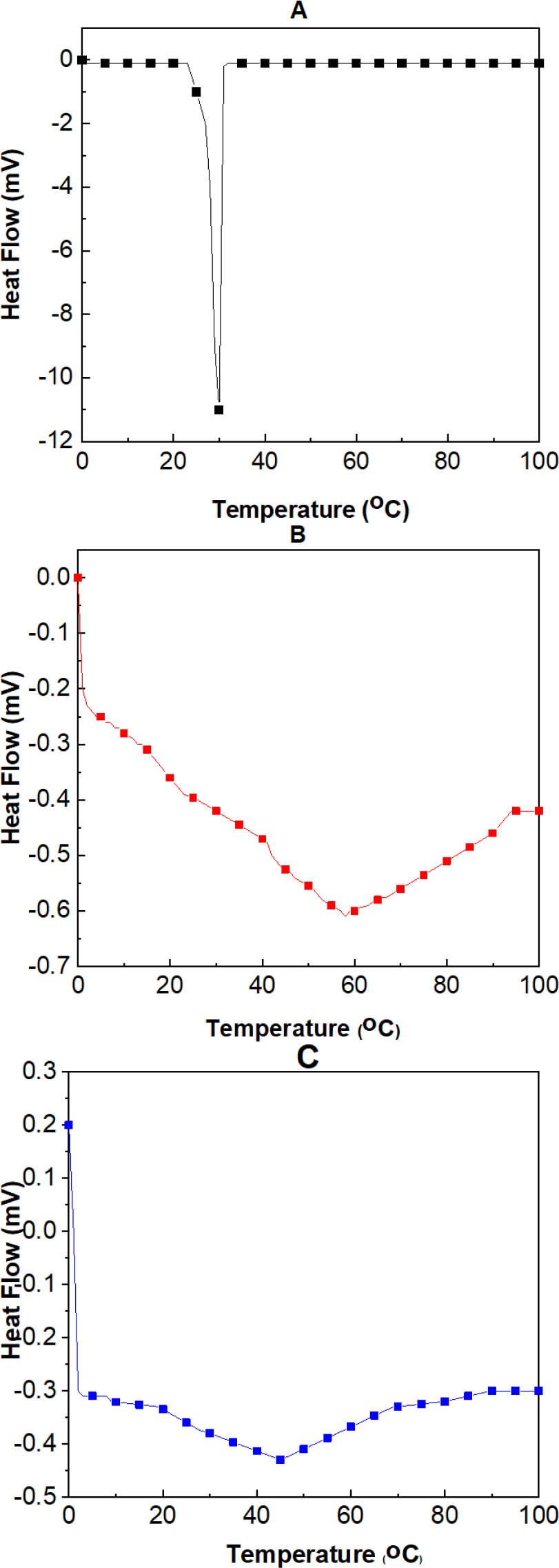
DSC Thermograms. (A) Drug free (FZN). (B) Blank (CSNPs). (C) Nanocomposite (FZNCSNPs). DSC, differential scanning calorimetry; FZN, fluphenazine
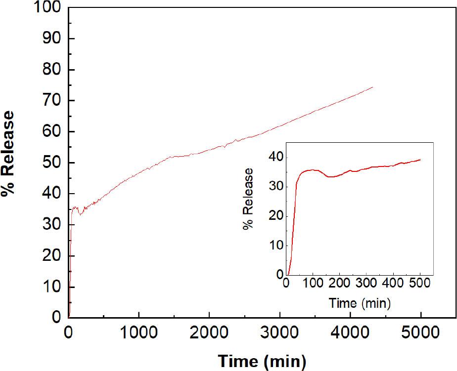
Figure 9 shows the FZN drug release profile from FZN-CSNPs nanocomposite into a solution of phosphate buffer saline (PBS) with pH 7.4. The drug release pattern out over 72 h (4,320 min) is divided into two stages; of these the first is an initial fast release, where 35% of the drug was released through 60 min. The initial burst release (i.e., at a rapid rate) from the CS NPs may be caused by the polymer’s swelling, creation of pores, or diffusion of the drug from the polymer’s surface [58].
In-vitro drug release study
In the second stage, the drug release becomes gradual in a slow pattern over the 3 days of the study. Forty-eight percent of the drug was released at the end of day 1, 62% at the end of day 2, and 74% at the end of day 3. The daily drug release rate indicated that it was relatively constant at the end of day 2, with around 12%. Thus, the drug needs at least 5 days to be completely released (100%). This sustained-release pattern improves patient compliance and adherence to the dosing by reducing the administration frequency and doses [59].
The XRD instrument was used to determine the crystal structures of powder materials. Figure 10A–D shows the XRD patterns of FZN, CSNPs, FZN-CSNPs nanocomposite, and physical mixture of FZN with CSNPs, respectively. Three strong diffraction peaks were observed in the FZN (powder) at the following 2θ of 17.3, 19.3, and 22.5 (Figure 10A).
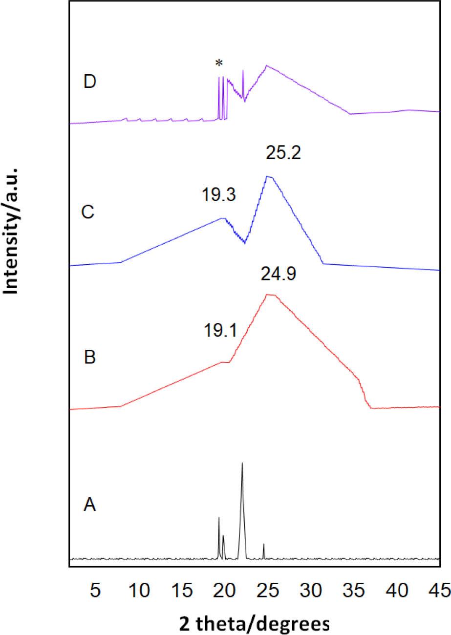
XRD-diffractograms. (A) Drug free (FZN). (B) Blank (CSNPs). (C) Nanocomposite (FZNCSNPs). (D) Physical Mixture of FZN with CSNPs. FZN, fluphenazine; XRD, X-ray diffraction
The diffractogram of CSNPs NPs at Figure 10B displayed two amorphous peaks at 2θ of 19.1 and 24.9 with a characteristic broad hump for the second peak [60]. The ionic interaction between TPP and protonated CS () leads to the formation of these CSNPs. The absence of any other diffraction peaks corresponding to impurities (such as TPP) were indicative of their purity. In FZN-CSNPs nanocomposite, however, no such crystalline peak of FZN was observed (Figure 10C). This result indicates that the FZN encapsulated in CSNPs is in the polymeric matrix’s amorphous form. This form of FZN inside the CS polymeric matrix produces benefits by ensuring sustained release of the FZN from the CSNPs NPs [61]. For the physical mixture of FZN and CSNPs at Figure 10D, all characteristic crystalline peaks of FZN were observed with less intensity (labeled as *), this result again confirming the amorphous properties of FZN in the nanocomposites [62].
Figure 11 demonstrates the chemical interactions between the three components (i.e., FZN, CS, and TPP) to form the FZN-CSNPs nanocomposites. The Fourier-transform infrared spectra of pristine FZN, CSNPs, and FZN-CSNPs nanocomposite are shown in Figure 12A–12C, respectively. The spectrum of FZN (Figure 9A) shows different absorption peaks; for example, the band at 3,200 cm−1 is related to the O-H stretching vibrations, while the band at 3,053 cm−1 is related to the C-H stretching vibrations of rings 1 and 2 (Figure 11). The band at 1,602 cm−1 was related to the stretching vibrations of C-S-C and C-C at rings 1 and 2. The bands at 1,240 cm−1 are related to the stretching vibration of C-H at rings I and II and also the stretching vibration of CF–3–[63].
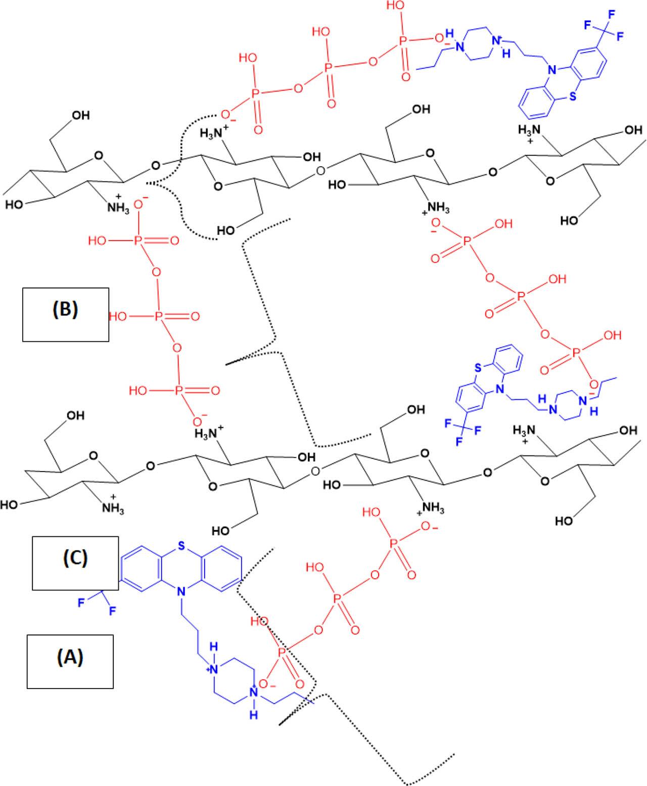
Chemical Interactions between the CSNPs and FZN drug. (A) FZN chemical structure. (B) CS chemical structure. (C) TPP chemical structure. CS, chitosan; FZN, fluphenazine; TPP, tripolyphosphate
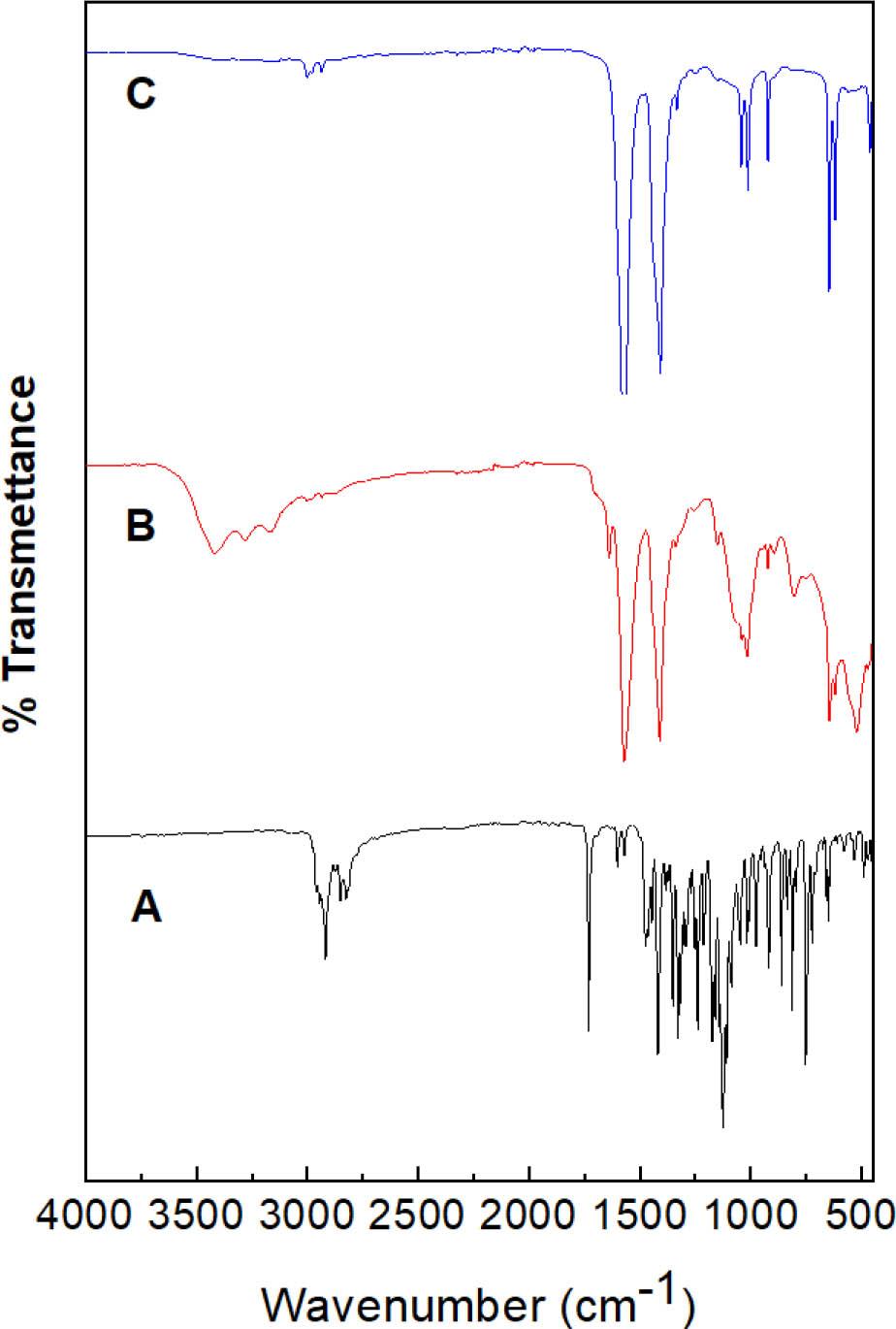
FTIR spectrums. (A) Drug free (FZN). (B) Blank (CSNPs). (C) Nanocomposite (FZNCSNPs). FTIR, Fourier-transform infrared spectroscopy; FZN, fluphenazine
The FTIR spectra of CSNPs is shown in Figure 12B. A peak at 3,418 cm−1 was observed for the main functional group of CS and is due to the O-H group of stretching vibrations. The presence of absorption peaks at 1,639 cm−1 and 1.573 cm−1 are due to the N-H bending vibration of the protonated amino (NH–2–) group and the C-H bending vibration of the alkyl group [64, 65, 66]. The absorption peaks at 1,039 cm−1 and 896 cm−1 are recognized due to the anti-symmetric stretching vibration of C–O–C bridges and assigned to glucopyra-nose ring in CS matrix.
FTIR spectrum of the FZN-CSNPs nanocomposite (in Figure 12C) shows the characteristic peaks for FZN, confirming that the drug was loading in the final formulation. For instance, the peaks at 1,243 cm−1 were due to C–H’s stretching vibration at rings I and II and stretching vibration of CF3. From Figure 11, it can be seen that FZN has protonated the nitrogen atom due to the pH condition of preparation. Therefore, the positive charge of FZN can interact with a negative charge of phosphate ions.
The present work highlights the DoE and NSGA-II optimization approach applications to provide mathematical models and propose an optimum formulation mixture with the best NPs size, ZP, and LE% for FZN-CSNPs nanocomposites as a drug delivery system. R-seq predicted regression models were 94.12%, 93.79%, and 91.61%, respectively. The three regression models were verified and validated using a test of hypothesis approach on a single mean, and the results enable us to conclude that the three models are fairly reliable and can be used as objective functions in further MOO analysis. Accordingly, NSGA-II has been employed to provide a set of optimum solutions in the Pareto front. One of the Pareto fronts was identified to be the trade-off points. Thus, the mixture parameters were optimized accordingly.
Further characterizations were carried out on the optimized formulation. Results of XRD, FTIR, and DSX indicated that FZN was successfully encapsulated. In-vitro drug release study indicated that full drug releases required at least 5 days. Consequently, the optimized formulation exhibited an extended-release pattern, can be used for long-term treatment, and could serve as a controlled drug delivery system model. Besides, the methodology utilized in this study creates a paradigm for future studies in the development and optimization of NPs drug delivery systems.
It appears that NPs delivery systems have a great potential to overcome some of the limitations in the conventional drug delivery system and in making drugs smarter. In the present work, the successful application of the DoE approach has been a critical tool in optimizing the FZN drug delivery system. Also, the effective utilization of the NSGAII approach was the solution to solve this kind of multiobjective problem. It was demonstrated that the three responses (i.e., NPs size, ZP, and LE) were statistically affected by the following NPs input fabrication process variables, i.e., FZN%, CS%, TPP%, and pH value. The findings suggested that those input parameters should be 13.3%, 64.2%, 22.5%, and 4.0%, respectively. On the other hand, the three responses were not statistically influenced by mixing time as a process variable.
Additional characterization studies on the optimized delivery system indicated that it exhibited an extended-release pattern, can be used for long-term treatment, and could serve as a controlled drug delivery system model. Hence, FZN, after optimization of its delivery system, could be effective in providing better treatment for schizophrenia. Ultimately, by manipulating some of the traits of NPs, researchers can improve the delivery system of important drugs needing to be released over a longer period of time, ensuring that these drugs can be administered with less frequent doses while ensuring the same bioavailability, which leads to increased adherence to treatment and reduced side effects as well. In addition, the methodology utilized in this study creates a paradigm for future studies in the development and optimization of NPs drug delivery systems.