Variability of chromatic vegetation indices derived from digital repeat photography in the Biebrza Valley

Introduction

Phenology is the science concerned with periodically recurring biological events in vegetation and animal activity (Lieth 1974). Understanding these cycles enables the prediction of seasonal ecosystem changes and their influence on the functioning of the biosphere. The value of tracking plant rhythms was recognised as early as ancient times, when simple observations supported the organisation of agricultural work (Piao et al. 2019). Systematic phenological monitoring began in the 18th century, with the establishment of permanent observation sites that laid the foundations for the first phenological networks (Koch et al. 2007). Early European pioneers include Robert Marsham and Carl Linnaeus (Koch et al. 2007; Strangeways 2018). However, the oldest known continuous phenological records come from Japan, where cherry blossom dates were documented as early as the 9th century (Aono & Kazui 2008).

Among the traditional approaches to phenological monitoring, manual field observations remain the most established and widely used. They involve direct monitoring of plant development by trained human observers, who record transitions between successive phenological phases. Detailed guidelines for conducting such observations are available (Koch et al. 2007). This approach provides high-resolution data specific to both the site and the observed plant species. It is particularly valuable in the context of ongoing climate change and its influence on phenology (Walther et al. 2002; Parmesan & Yohe 2003; Richardson et al. 2013), which has led to its recognition as an essential biodiversity variable (EBV) (Pereira et al. 2013). However, a major limitation is the restricted spatial coverage achievable by individual observers. Piao et al. (2019) also point out challenges related to uneven geographic distribution of observations, limited ecosystem representation and logistical difficulties in remote or harsh environments.

While manual observations provide highly detailed, site-specific data, technological advancements have enabled broader-scale vegetation monitoring through remote sensing techniques. The development of satellite measurements has led to the widespread use of vegetation indices. Among the most popular are the Normalised Differential Vegetation Index (NDVI), Extended Vegetation Index (EVI), Leaf Area Index (LAI) and Solar-Induced Fluorescence (SIF), all of which have proven effective across a wide range of ecosystems (Duchemin et al. 2006; Garrity et al. 2011; Mohammed et al. 2019; Gerard et al. 2020; Zeng et al. 2021; Zhou et al. 2022). These methods allow for the monitoring of large and remote areas inaccessible to human observers. However, they are subject to limitations such as atmospheric interference, which can affect data quality and availability. Furthermore, the increased spatial coverage comes at the expense of lower measurement resolution. Land surface phenology typically aims to determine the start, peak and end of the growing season (SOS, POS, EOS) (Misra et al. 2020). A significant limitation remains the issue of mixed vegetation within a single satellite pixel, which remote sensing methods are unable to distinguish (Richardson et al. 2018).

Phenocamera systems combine the advantages of both manual and remote phenological monitoring methods. They involve the use of standard digital cameras installed at fixed locations to capture images at regular time intervals (Richardson et al. 2007). This approach enables automated, remote data collection, while still allowing for visual inspection and the manual extraction of phenological event dates. Furthermore, the acquired images can be processed in a similar manner to those from satellite data, providing quantitative information about image colours from which vegetation indices may be derived (Richardson 2019). Among the most widely used are RGB chromatic indices, which offer a simple and effective means of tracking vegetation development through changes in colour saturation (e.g. Migliavacca et al. 2011). When equipped with infrared-sensitive sensors, phenocameras also enable the calculation of more advanced indices such as NDVI (e.g. Petach et al. 2014).

The increasing popularity of phenocameras and the digital repeat photography method is reflected in the emergence of dedicated monitoring networks. These include PhenoCam (Richardson et al. 2018), EUROPhen (Wingate et al. 2015) and the Phenological Eyes Network (Nasahara & Nagai 2015), which continuously collect images at observation sites. Many of these are co-located with eddy covariance (EC) towers measuring greenhouse gas fluxes, allowing researchers to integrate biotic factors into assessments of the terrestrial carbon cycle (Peichl et al. 2015). In Poland, phenological monitoring is carried out by the Institute of Meteorology and Water Management – National Research Institute (IMWM-NRI), primarily through manual observations at 51 synoptic stations. Between 2013 and 2017, IMWM-NRI implemented a pilot programme in cooperation with the Polish Grid Infrastructure PL-Grid and the Poznań Supercomputing and Networking Centre, aimed at developing a system for remote phytophenological observations (Mager & Kępińska-Kasprzak 2015). Separately, a recent study by Różańska et al. (2025) presents the application of digital repeat photography and the analysis of vegetation indices, marking one of the first scientific uses of this method in Poland.

The aim of this study is to analyse vegetation development in a temperate wetland ecosystem (Biebrza National Park, north-eastern Poland), using chromatic indices derived from digital repeat photography during the 2022–2024 period. Specifically, the study objectives are: (i) to present the annual patterns of chromatic indices, (ii) to compare their values across the consecutive years of the study period and (iii) to interpret the observed variability in relation to meteorological conditions.

Research area

The research site is located in the Middle Biebrza Basin, within the Biebrza National Park (53° 35′ 30.8″ N, 22° 53′ 32.4″ E), approximately 350 m north of the village of Kopytkowo (Fig. 1). At a distance of 4–8 km to the north and north-west lies the ‘Red Bog’, a strict protection area preserving the valley's original character. The immediate surroundings of the research station are characterised by the presence of the Kopytkówka River, although its exact course is difficult to determine due to dense reed vegetation overgrowing both the riverbed and the adjacent areas.

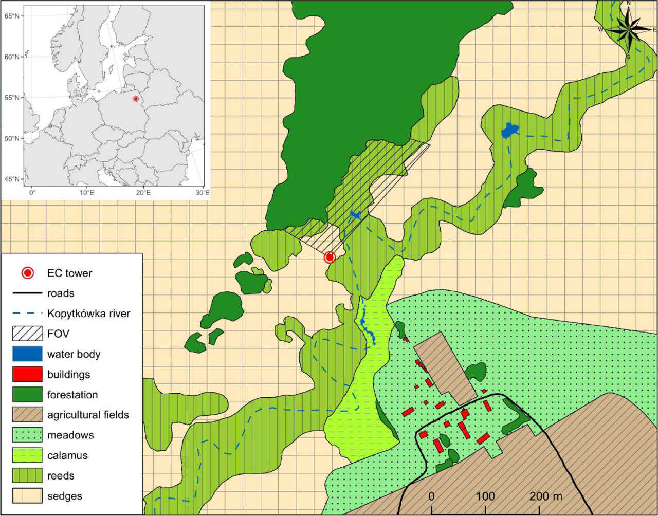
Figure 1.

The dominant vegetation at the site includes Phragmites australis, Acoretum calami, Carex rostrata and Thelypteris palustris (Fortuniak et al. 2021). These species are known to follow the C₃ photosynthetic pathway (Pagter et al. 2005; Stofberg et al. 2015). The Biebrza Valley lies within a temperate climate zone with both continental and oceanic influences. For the reference period, 1991–2020, the mean annual air temperature was 7.3 °C and the average annual precipitation totalled 557 mm, based on data from the IMWM-NRI meteorological station located 22 km north-west of the study site (ID: 253220070, Biebrza-Pieńczykówek).

The area of the Middle Biebrza Basin along the Kopytkówka River includes peatlands, the soils of which have been partially degraded due to drainage. The peat structure in this region is dominated by reed and sedge peat at medium to advanced stages of decomposition (Fortuniak et al. 2017). The growing season, defined as a period with mean daily temperature ≥ 5 °C, lasts approximately 210 days in this part of Poland (Tomczyk & Szyga-Pluta 2016).

Methodology

A NetCam SC camera (model SD500BN, StarDot Technologies, USA) was mounted in March 2022 on a mast at the Kopytkowo station to measure energy and greenhouse gas exchange using the eddy covariance method (Fig. 2A). The camera was placed in a protective enclosure at 4.7 m above ground level, facing north to minimise the impact of direct sunlight on exposure and to reduce variations in image brightness during the day (Fig. 2B). Images were taken every 15 minutes between 4:00 and 23:00 and saved locally in JPG format as 24-bit images at a resolution of 2592 x 1944 pixels. The collected images were visually inspected to ensure camera stability and avoid potential frame shifts.

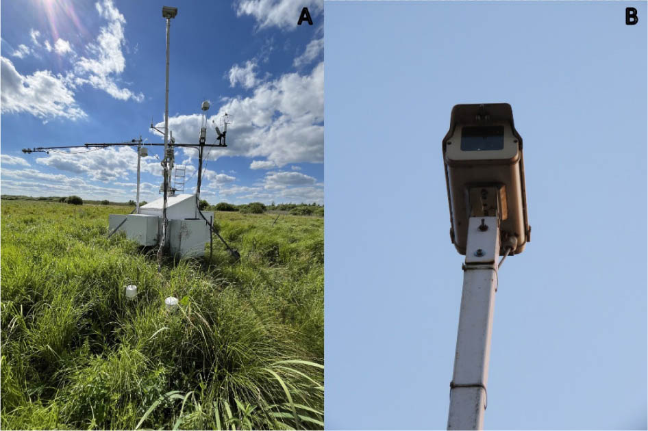
Figure 2.

The chromatic coordinates of the RGB model were calculated to normalise the contribution of each colour channel, according to the following formulas:

To obtain chromatic coordinates, the phenopix package for the R environment was used, which enables image processing, visualisation of the greenness indices and extraction of phenological metrics (Filippa et al. 2016; Filippa et al. 2024). All calculations were performed using R Statistical Software (R Core Team 2023). The first step of the analysis involved defining a region of interest (ROI), within which the digital number values of each channel were extracted for every pixel. In this study, a single, large ROI was selected to encompass all vegetation visible within the camera's field of view but located below the horizon line (Fig. 3); this was to avoid overestimation of the blue channel due to the presence of sky. The selected ROI included vegetation dominated by reed and sedge species. This approach helped minimise the influence of local variations in lighting changes (e.g. shadows or light reflection), and allowed for averaging of phenological signals from both plant groups to represent overall greenness dynamics. To ensure consistency and avoid potential bias from reselecting the ROI, the same region was applied across all analysed years.

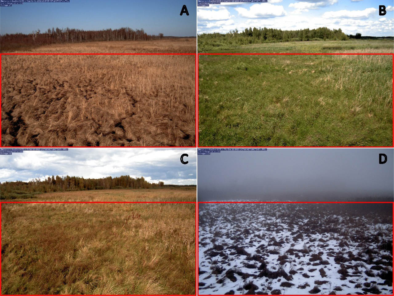
Figure 3.

The next step involved extracting RGB colour information using a built-in function from the phenopix package. This process consists of averaging the values of vegetation indices across the defined ROI, resulting in a time series of mean intensity values for the red, green and blue channels. To ensure the reliability of the results, values derived from images captured before sunrise and after sunset were excluded from the analysis. The exact times of these solar events were calculated based on the geographical coordinates of the measurement station using the suncalc package (Thieurmel & Elmarhraoui 2022).

The final computational step involved recalculating the chromatic components (Eq. 1a, 1b and 1c). To minimise the impact of variable scene illumination caused by changing atmospheric conditions, the data were subsequently filtered. Specifically, a moving 90th percentile filter was applied over a three-day window, with the resulting value assigned to the central day of the window (Sonnentag et al. 2012). It is worth noting that due to a power outage in 2023, a gap of several days occurred in the chromatic coordinates, coinciding with the June peak of plant activity.

Temperature data, acquired from a measuring station using an HMP60 temperature probe (Vaisala, Finland) positioned 2 m above ground level, were also used in the analysis of chromatic indices. Based on these data, growing degree days (GDD) were calculated by averaging the minimum (T_min,i) and maximum (T_max,i) daily temperatures and subtracting a base temperature (T_base = 10 °C). If the resulting average was below 10 °C, the GDD value for that day was set to 0 (Eq. 2a). Annual growing degree day sums (GDDS) were then obtained by summing daily GDD values from the beginning (i) to the end (j) of the summation period (Eq. 2b).

Results

The obtained values of the chromatic indices show features of seasonal repeatability, which becomes clear when the course of the annual values is visualised. Figure 4A shows the r_cc index. Its values remain relatively stable over the course of each year. The greatest variability is observed in the early and late part of each year, particularly for 2024, when a significant decrease in values appeared. During the spring period, values range between 0.45 and 0.50, with little variability between the years studied. Differences begin to appear in April with the arrival of the growing season, when a gradual decrease in the index values begins, until the minimum values for this period are reached in June. Here, the greatest differences between the years are marked, with 2024 taking on the lowest values of the period under study. After mid-June, a gradual and sustained increase in the indicator begins, until the maximum values for each year are reached in October.

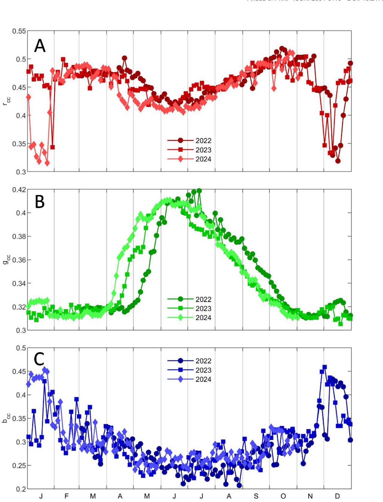
Figure 4.

The g_cc index maintains its values at around 0.32 for around half of the year (Fig. 4B). An increase in value was recorded in April, which coincided with a decrease in the r_cc value. It is clear how the timing of the increase in the indicator changes from year to year. A clear difference can be seen between 2022 and 2023. In 2024, the increase starts as early as the end of March. At the same time, the peak in vegetation activity, which had been shifting from year to year, is also shifting. After the June maxima, the values gradually decreased until they stabilised again at the beginning of November, when they again oscillated around 0.32.

The b_cc index shows the opposite course to the g_cc values (Fig. 4C). Its highest values were recorded in the winter months, with clear peaks in January and December when it reached around 0.45. In the following months, the values decrease as spring progresses, until they reach their minimum values in mid-summer when b_cc were recorded at 0.20–0.25. In the second half of the year, there is a slow increase in values until a second peak is reached at the end of the year. For this index, it is during the winter period that the greatest discrepancies between the years studied occur, particularly for 2024, when higher b_cc values were recorded than in the corresponding days of the other two years.

The temperature course over the study period followed a typical seasonal pattern, with the lowest values recorded in winter and the highest in summer (Fig. 5). Nevertheless, clear differences between the years are apparent. The year 2024 was the warmest of the three, characterised by the earliest and fastest rise above 5 °C, marking the onset of the growing season. In contrast, air temperature declined most rapidly in 2022, with a clear drop observable from August onwards, continuing until the end of the year.

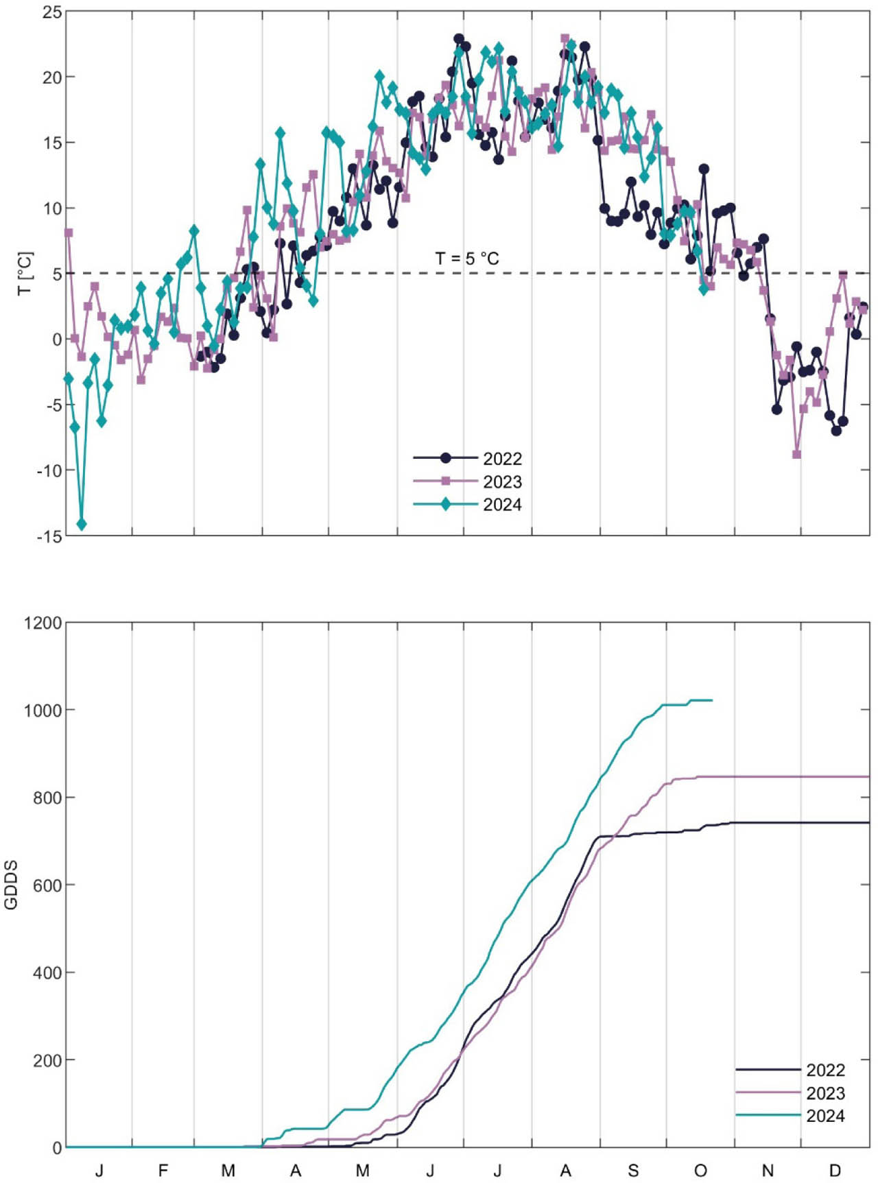
Figure 5.

This is also clearly reflected in the GDDS trajectories, which show how cumulative thermal values progressed over the course of each year. The steepest increase occurred in 2024, beginning as early as April and continuing through September, ultimately resulting in the highest total – exceeding 1 000. A similar accumulation pattern was observed in 2023, though it started slightly later than in 2024 and reached a lower final value.

Discussion

Chlorophyll is the pigment responsible for the green colour of plants (Palta 1990). Since it absorbs most wavelengths of visible light while reflecting green light to a greater extent, plant parts containing chlorophyll appear green to the human eye (Virtanen et al. 2022). Its primary role is to absorb solar radiation and convert it into chemical energy during photosynthesis. Consequently, chlorophyll concentration is often used as an indicator of plant development and physiological status (Gitelson et al. 2003). This relationship forms the basis for using digital repeat photography as a non-invasive tool for monitoring vegetation dynamics.

Studies using digital repeat photography reveal the seasonal dynamics of chromatic index values (Fig. 4). The highest g_cc values were observed in summer, with a distinct peak in June, while the lowest values occurred in winter. This pattern corresponds to the typical vegetation activity cycle of the temperate climate zone. An increase in g_cc was first recorded in April, aligning with the onset of the growing season in this region as defined by the thermal criteria (Tomczyk & Szyga-Pluta 2016). Similarly, the peak g_cc values in June coincide with the beginning of the maturation phase, which is also determined based on daily temperature data (Tomczyk 2022).

Although the seasonal pattern of g_cc change was similar across all study years, noticeable interannual differences were evident in the timing of onset, the rate of increase and the maximum values of the index. In 2024, g_cc values began rising earlier than the two previous years, coinciding with an earlier exceedance of the 5 °C daily mean temperature threshold and the highest total GDDS recorded over the entire study period (Fig. 4B, Fig. 5). In contrast, g_cc values in 2022 increased later, reflecting delayed thermal accumulation. A comparison between 2022 and 2023 further illustrates the influence of GDDS on vegetation dynamics, with 2022 values surpassing those of 2023 from early July onwards, which was directly reflected in higher g_cc values for that period. This behaviour is characteristic of C₃ plants, whose photosynthetic efficiency is strongly influenced by air temperature and water stress (Ehleringer 1978; Pagter et al. 2005).

Seasonal variation was also evident for the remaining chromatic indices. The r_cc values exhibited an inverse pattern to those of g_cc, reaching a peak towards the end of the growing season when vegetation activity declined. Red pigmentation in plants is primarily due to carotenoids and anthocyanins (Tanaka et al. 2008). These compounds play important photoprotective roles, particularly in safeguarding the photosynthetic apparatus from excess light stress via mechanisms such as the xanthophyll cycle (Gamon & Surfus 1999; Ruban & Horton 1999). Short-term peaks in r_cc observed during the summer months may be associated with the activation of this protective process. As plants age over the course of the growing season, chlorophyll content typically declines while carotenoid levels rise, resulting in characteristic shifts in leaf coloration (Keskitalo et al. 2005; Lichtenthaler 1987). This phenomenon was clearly reflected in the temporal pattern of the r_cc index (Fig. 4A). The abrupt drops in r_cc values observed at the beginning and end of each year coincided with simultaneous increases in b_cc, likely reflecting the presence of snow cover. The subsequent trajectory of the b_cc index was largely driven by rising g_cc values, which reduce the relative contribution of the other colour channels.

The key role of temperature in shaping the seasonal course of vegetation indices observed in this study is consistent with findings from previous research. Several studies have highlighted temperature as a critical driver of phenological changes and greenness dynamics in various ecosystems (Linkosalmi et al. 2016; Linkosalmi et al. 2022; Peichl et al. 2015; Richardson et al. 2019). These studies show that the higher spring temperatures often lead to earlier green-up and increased photosynthetic activity, whereas delayed warming slows the onset of the growing season. The interannual differences observed in this study, especially the early rise in g_cc in 2024 in response to faster thermal accumulation, reflects this well-documented phenomenon. However, many of these studies also highlight the role of other abiotic factors, which can modulate plant response to the environment. This signifies the need for further, more complex analysis.

Conclusions

The aim of this study was to analyse vegetation development in the unique wetland ecosystem of the Biebrza National Park, recognised as a site of European importance, using digital repeat photography. The method proved effective in capturing both seasonal and interannual variations in chromatic indices, demonstrating its potential for future long-term monitoring and ecological research.

The g_cc values displayed a clear seasonal pattern, with the highest values recorded in June, aligning with the thermal growing season as defined by established criteria. This indicates that the accuracy of the chromatic indices is sufficient to support their use in further environmental analyses. Notable differences between the studied years reflected variations in air temperature and GDDS, underscoring the strong influence of thermal conditions on vegetation development.

Other chromatic indices also provide insights into phenomena such as snow cover presence or plant water stress in the study area. However, the method's limitations – stemming from the interdependence of chromatic indices – should be taken into account. While a strong relationship between air temperature and g_cc was confirmed, the potential influence of other abiotic factors on vegetation dynamics should not be overlooked, highlighting the potential for future studies.