
Introduction
Rising economic inequalities have attracted much attention in political circles. Indeed, tackling inequalities has been presented as a political imperative for the European Commission (EC 2015); as integral to achieving the Sustainable Development Goals by the United Nations (UN n.d.); and as an important basis for sustained long-run growth by the OECD (Cingano 2014). At the same time, as a much-debated book by Thomas Piketty (2014) clearly illustrates, the topic has sparked intense discussions among academics (see, for example, Acemoglu & Robinson 2015; CESifo 2015; Kopczuk 2015).
As a result of this increased interest, a lot of new research has focused on economic inequalities. While our knowledge about the distributional landscape has been constantly improving, our understanding of the determinants and consequences of the unequal distribution of economic resources is still limited. This is largely due to the lack of reliable data. In fact, inequalities have many aspects but some of them are poorly measured, if at all. Furthermore, the existing datasets (that use, for example, surveys or tax data), while being very useful, have various problems related to potential sampling bias or tax evasion (see, for example, Kopczuk & Zwick 2020).
Not surprisingly, therefore, researchers persist in their efforts to provide new ways, either direct or indirect, to improve our knowledge about economic inequality, its extent and trends, as well as its causes and potential consequences for the future. Interestingly, in terms of geographical distribution, these efforts have been highly uneven. Indeed, while for some countries we have a much more precise picture of the level of wealth/income concentration and how it evolved over time, for others, we have a much poorer understanding of what has happened and why. One country for which we still have a very incomplete insight into the issue of inequality is Poland (Obserwator Finansowy 2020). Thanks to some recent contributions to the literature (Brzeziński et al. 2020; Brzeziński & Sałach 2021; Bukowski & Novokmet 2021), this has been slowly changing. Nevertheless, for many distributional aspects, we still need to achieve a much better understanding.
One issue, on which we have only limited evidence, concerns the level of inequality in Poland’s rural areas. While this could probably be explained in a variety of ways, two factors certainly appear to play a role. First, a predominant share of GDP in Poland, as elsewhere, is generated in urban centres (MRR 2010; OECD 2019). In consequence, if the aim is to capture the distribution of income, it may seem an obvious to focus on urban areas. Second, and relatedly, rural areas, especially those located further away from large metropolitan areas, continue to be dominated by agricultural activity, despite the ongoing process of deagrarianisation (Halamska & Stanny 2021). This is important in the context of investigating inequalities because farmers in Poland do not pay personal income tax. 1 As a result, any analysis based on tax data will likely omit this social group.
While such an omission might be justified in some cases, in general, directing our focus on the non-farming population has a number of important shortcomings. One obvious consequence is that we lose sight of a significant number of households. It is worth noting that this is not a marginal issue. Indeed, according to data from the agricultural census conducted in 2020, the number of farms has been estimated at approximately 1.3 million. In addition, there is a risk that the wealth/income of this group may be severely underestimated if calculated solely on the basis of (part-time) off-farm employment, assuming that the latter can be elicited from the tax data. A second consequence of omitting farmers is that an important factor that affects the level of wealth – namely land – is excluded from the analysis. Given the fact that agricultural land accounts for just under 50% of the country’s area (Wilkin 2019), to not include it in the analysis can be seen as a significant drawback. Therefore, taking a more detailed look at farmers might be a way to draw wider implications for our understanding of economic inequalities in Poland and especially in rural areas.
In response to these concerns, we present a new dataset on the distribution of income support in rural Poland in this paper. This was constructed on the basis of records of all individuals who receive funding from the European Union’s Common Agricultural Policy (CAP). The dataset covers the period 2014–2021 and, thus, it offers the possibility of documenting the changes in the distribution of total income support granted to land users over time. The dataset provides information aggregated at the municipality level (i.e. LAU level, according to Eurostat). Hence, it is suitable for all sorts of regional analyses.
Advantages of the new dataset
The new dataset offers several advantages. First, as already mentioned, it specifically concentrates on farmers – a group that often escapes the attention of researchers. As such, it allows users to either focus on the group itself or merge the data on farming population with other datasets (covering different sub-populations), thus making it possible to take a broader view on distributional issues.
Second, the presented dataset can be used to analyse both income and wealth distribution. Indeed, the most common way to look at CAP support is to treat it as a form of income support (EC n.d.). In effect, the presented dataset, especially combined with FADN data, which allows the share of total income support in farmers’ incomes to be calculated, may be used to take a closer look at the distribution of the latter. 2 That said, and importantly, our dataset might also provide useful insights into wealth inequality, which has become a central concern in a large part of the literature (Piketty 2014). Capturing this information is possible because, for part of the support (often referred to as direct payments), the Single Area Payment Scheme (SAPS) is used in Poland. In SAPS, the support paid is based solely on the number of eligible hectares declared by farmers and the level of support is the same for all hectares in the country. In effect, the distribution of single area payments in Poland may serve as a good approximation of land use distribution 3 and, thus, given the fact that land could be seen as an important asset in many rural areas, be informative on wealth inequality. This feature of our data corresponds very well with the recent contributions to the literature claiming that a (large) part of wealth may arise precisely from land (Artola Blanco et al. 2021; Bonnet et al. 2021). In this context, it might be worth mentioning that from 2010 to 2020, which roughly corresponds to the period covered by our data, nominal agricultural land prices in Poland have almost tripled. 4 This, in turn, suggests that having access to land might have been an important factor behind wealth accumulation in Poland.
Third, the dataset provides information at municipality (gmina) level. This appears to be an important advantage over other datasets, which report various inequality measures at country level. Thanks to this, researchers can take a much more detailed view on the potential heterogeneity in the level of, and changes in, income/land inequalities. Obviously, if needed, our data can be used for analyses at more aggregated (county – powiat, subregion or voivodeship – województwo) levels. This presents a big difference between our dataset and FADN data. The latter, in principle, also includes information on farm payments at individual level. However, it is based on a surveyed sample and cannot be used at the municipality or county level (due to an insufficient number of observations). 5
Fourth, the dataset allows various inequality measures to be examined and is not limited to the Gini index, which has often been used in other research focusing on land inequality (Deininger & Squire 1998). While being useful, the Gini index has its shortcomings (for example, the same Gini index may be observed for two regions even though their asset distribution is different). It is important, therefore, to complement this with other inequality measures. In particular, with our data, one can easily measure higher-order moments (e.g. skewness, kurtosis), analyse income support shares – namely the share of support granted to a given population group such as the top 1%; top 10% or bottom 10% (see, for example, Piketty 2014; Kopczuk & Zwick 2020 – for analyses of various types of income data; or Bauluz et al. 2020 – for the work on land distribution) or other commonly used measures, such as the Theil index, Atkinson index or the coefficient of variation (Davies et al. 2017).
Fifth, the dataset covers the whole population of farmers receiving income support, which is roughly 1.3 million records per year. Therefore, in contrast to many other datasets focusing on inequalities, our data is free of potential concerns related to relying only on one or another segment of the population of interest. Furthermore, and relatedly, the data includes farmers at both ends of the distribution: those who receive the least and those who receive the most. What follows is that the data should accurately capture the very bottom and the very top of the distribution (see, however, some caveats listed in the next section).
Sixth, the dataset does not rely on farmers’ declarations but is based on official records documenting all payments that were made. Accordingly, we do not have to worry that some payments were not reported (misreported) or that the reports on payments for some categories of farmers (richest, poorest, with or without political connections, etc.) are biased (for example, rich people are often reluctant to reply to surveys measuring incomes/wealth). Thanks to this, typical concerns related to surveys measuring the level of economic inequalities do not apply.
Seventh, the fact that the municipality-level aggregates are based on individual data implies that we do not have to make any imputations and the resulted measures are not estimates (which can vary in accuracy). Likewise, we do not have to make any a priori assumptions about the underlying population/asset ownership/income.
Eighth, the fact that some of the support is paid per hectare provides an opportunity to complement the picture that emerges from other datasets that measure land distribution – either by extending the period of analysis or by taking a closer look at differences/similarities in changes in land distribution depending on the data used. A natural point of reference here is the data collected during agricultural censuses in 1996, 2002, 2010 and 2020.
Ninth, in addition to information on individual farmers, our dataset also contains information on financial transfers to institutional beneficiaries 6 (legal persons, unincorporated entities, civil partnerships). This allows any changes in the importance of the latter in income support/land use distribution at the local level to be traced. That said, as mentioned in Section 2.1 below, this data should be treated with caution as it displays huge variability between years. The dataset is constructed in such a way that a particular type of beneficiary can be included or excluded, depending on the research interest.
Finally, although the dataset is most suitable for capturing inequalities in rural municipalities with a relatively large dependence on agriculture, it includes data for all beneficiaries, including those residing in urban or urban–rural municipalities. In consequence, the data might be useful not only for researchers with a primary focus on rural areas/agricultural economics but also for those interested in the processes of urban sprawl, rural–urban migrations or the role of agricultural holdings in determining the wealth of urban dwellers.
Data issues that should be kept in mind during the analysis
While the presented dataset has several advantages, it is not without its problems. The following data issues should certainly be taken into account while using the dataset. First, some municipalities have a fairly small number of income support beneficiaries. Indeed, in some cases this number is lower than 100. The researcher should, therefore, judge whether these municipalities should be included in their analysis. It is important to note that, for each municipality, the dataset provides the number of beneficiaries included in the inequality measures; researchers can therefore easily adopt any cut-off point according to their own needs.
Second, some municipalities are not included in the data. This is due to the fact that, in the original dataset, published by the Ministry of Agriculture and Rural Development, only information on the name of the municipality and the postal code was made available. In several cases, however, the names of rural and urban municipalities were the same, and the postal code information was not enough to distinguish one from the other. For a detailed description of this issue, see the discussion in the next section.
Third, while our data offers a good opportunity to analyse various issues related to land distribution, it is important to note that land, although being an important asset, may constitute just one element of the wealth of people living in rural areas. This needs to be taken into account if the dataset is to be used for analysing the distribution of wealth.
Fourth, and relatedly, it needs to be kept in mind that our dataset includes only land that is used by the people who receive direct payments. While it is reasonable to assume that all people who are eligible for these payments apply for them, according to the current regulations, the users of the smallest holdings – those below one hectare – cannot be paid. 7 In consequence, extremely small farms are not included in the dataset. In order to assess how important that omission is, the two following pieces of information might be helpful. On the one hand, according to the most recent Agricultural Census conducted in 2020, the total number of farmers in Poland is 1.3 million, and approximately 25,000 farmers have less than one hectare. 8 From this angle, therefore, our dataset includes approximately 98% of farmers. On the other hand, the total agricultural area in Poland is 14.9 million hectares (GUS 2022). According to the Agency for Restructuring and Modernisation of Agriculture – designated to perform the role of an accredited paying agency – the direct payments area amounts to approximately 14.3 million hectares (ARiMR 2021b). Taken from this view, our dataset accounts for 96% of the agricultural area in the country. Overall, then, our dataset appears to cover almost all agricultural land and almost all farmers in Poland.
Fifth, and still relatedly, our data captures land use distribution rather than land ownership distribution. From the distributional point of view, the latter might appear to be more important. That being said, our data can still be informative. To see this, one should refer to research conducted by the Institute of Agricultural and Food Economics (IERiGŻ 2018). According to the estimates presented there, in 2017, the share of farms using leased land (farmer-to-farmer rentals) was around 20%, and leased land (through private rentals) accounted for, on average, around 15% of the cultivated area. Apart from that, around one million hectares of public agricultural land was rented, which roughly accounts for an additional 7% of the cultivated area. 9 This clearly shows that tenancy, although being used, is much less prevalent than land ownership. That said, the incidence of tenancy is likely to vary across regions/municipalities. Hence, drawing conclusions about land ownership on the basis of our data may not be easy.
Sixth, and relatedly, as the largest landowners artificially transfer the land to family members, our data may underestimate the level of land use concentration. Put differently, while calculating inequality measures at municipality level, we treat every individual beneficiary equally. Consequently, we do not take into account the possibility that one person may also effectively operate land that is registered under different names (e.g. family members).
Seventh, when using our data to make comparisons between years, one should rely on relative measures rather than comparing changes in absolute values. This is because payment rates varied over time. In addition, the EU support for farms has evolved over the years. For example, new forms of support have been introduced and the amounts paid under the old measures have decreased.
Eighth, and relatedly, since 2016, Poland has applied the Small Farmers Scheme (SFS), granting a one-off payment to farmers whose income support payments do not exceed EUR 1,250. 10 This replaced all other forms of income support payment for this group. In consequence, for these farmers, we can no longer differentiate between single area payments and other payments. This makes it impossible to accurately determine the acreage cultivated by farm households in this group. Nevertheless, we believe that our data can also serve as a good approximation for land use for these farmers. This is because the data suggests that, among farmers who joined the SFS, the one-off payment (paid from 2016 onwards) seems to largely correspond to the single area payment that they received in 2014 and 2015. We base this belief on the following observation. Among farmers who joined SFS, the share of the one-off payment in total support oscillated between 75–85% between 2016 and 2021. This is very close to the 81–82% share that the single area payments accounted for in total subsidies for this group of farmers in 2014 and 2015. 11 In consequence, it does not appear that we are making a big mistake in assuming that SFS payments represent the equivalent of single area payments.
Ninth, data on institutional beneficiaries shows a suspiciously high degree of variability between years. This relates to the number of such beneficiaries, the amounts they received, and the share in total payments. For example, we observe a huge decrease in the latter between 2016 and 2017, despite the fact that the data suggests an increase in the number of institutional beneficiaries in this period. The year 2019 also seems to stand out in this respect (see Tables A1 and A2 in the online Appendix). 12 Overall, this problem appears to be more acute in cases of data on total payments than on single area payments. That said, when using this data, regardless of the type of payments, one needs to be cautious.
With these advantages and shortcomings in mind, we now present detailed information on how the dataset was constructed.
Description of the dataset
The dataset, available at https://beneficjenciwpr.wne.uw.edu.pl, contains annual data on income support for farmers at the municipality level for the period 2014–2021. The source data was scraped from a website operated by the Polish Ministry of Agriculture and Rural Development (https://beneficjenciwpr.minrol.gov.pl/). The website presents information on all beneficiaries of the European Union’s Common Agricultural Policy in Poland. 13 Our focus is on the distribution of two types of payments. On the one hand, we are interested in the distribution of single area payments – referred to as measure I.2 in the description of the support schemes set out in Annex I to Regulation (EC) 73/2009 of the Council. 14 As argued earlier, this can be informative with regard to the distribution of land use, as the payment for eligible agricultural land is based on a flat rate (the same rate is applied countrywide). On the other hand, we focus on the distribution of total payments – the sum of all payments listed in the above-mentioned Annex – received by CAP beneficiaries. While single area payments are the most important form of subsidising farmers in Poland, CAP payments include other support measures. A look at total payments, therefore, allows for a broader picture; if the analysis is not limited to land use distribution, this might be more useful.
We collected the data and filtered it in the source website by name of municipality; when needed, we used additional filtering based on the payment amount. 15 In this way, we calculated a total number of 10,989,718 beneficiaries for the 2014–2021 period, including both individuals and institutions. We removed 41 observations that had missing postal codes, missing names and missing data on received payments (11 in 2015; 6 in 2016; 24 in 2018). Another 28,229 beneficiaries received zero payments (27,379 in 2016; 20 in 2017; 830 in 2018) and were also removed from the source data. Given the fact that some beneficiaries received only very small amounts, we decided to apply an additional filter when calculating inequality measures by excluding observations whose total payments were less than PLN 750 (~ EUR 190). The reason we adopted this threshold was that lower payments were extremely rare (irrespective of the year in question). This can be clearly seen in Figure A1, presented in the online Appendix. This filter resulted in excluding 22,328 beneficiaries from the calculations (from 1,511 in 2015 to 4,266 in 2017). In the end, we considered 10,939,120 beneficiaries – approximately 1.3–1.4 million for each year.
The vast majority of these beneficiaries are individual farmers, with institutional beneficiaries accounting for 0.7–1.2% of these. However, the share of the latter in the amounts of direct payments received is much higher. On average, this was 17.4% – the figure decreased from 24–25% at the beginning of the period to 12–13% in recent years.
As mentioned above, since 2016, the Ministry of Agriculture and Rural Development has applied the small farmers scheme (SFS), granting a one-off payment to farmers whose income support payments do not exceed EUR 1,250. 16 At the beginning of the period, this type of beneficiary accounted for approximately 54% of individual farms receiving the payments. Over time, however, this share has decreased and, in 2021, it amounted to 42%. The exact number of observations assigned to each category of beneficiaries is presented in Table A1 in the online Appendix.
The total value of all payments received by beneficiaries in the analysed period amounted to PLN 183 bln, ranging from 19 to 27 bln in particular years. At least half of these payments (49–64%, depending on a year) were single area payments, amounting to PLN 98 bln in total – a range of 12–13 bln every year. The average total payment received by small farms participating in the SFS amounted to approximately PLN 3,000 each year (with a median of about PLN 2,400). The respective amount for the remaining individual farmers (not participating in the SFS) was, on average, about PLN 22–27,000 (with a median of PLN 12–13,500). A huge majority of this type of beneficiary (92–98%) received single area payments, which accounted for 52–67% of their total payments on average. The average payment for institutional beneficiaries, in turn, exceeded PLN 300,000 17 and only 40–63% of them received single area payments. In most years, the average single area payment for this type of beneficiary accounted for 40–45% of the average total payment. Table A2 in the online Appendix presents the relevant statistics for different types of beneficiaries, focusing on those residing in rural municipalities and receiving at least PLN 750.
One issue that had to be resolved when compiling the dataset was that, in Poland, 470 municipalities do not have a unique name. Consequently, individual beneficiaries could not always be unambiguously assigned to a given administrative unit. In the vast majority of cases, a municipality was repeated twice (428 municipalities, 214 names), eleven municipality names were repeated three times (Czarna, Baranów, Bolesławiec, Brodnica, Brzeziny, Kolno, Lipno, Oleśnica, Poświętne, Sławno, Świdnica) and two four times (Dobra, including Dobra (Szczecińska) and Osiek). Among the municipalities with non-unique names, 156 pairs consisted of an urban municipality and the surrounding rural municipality of the same name (see Table A3 in the online Appendix for the list of these pairs of municipalities). Whenever it was possible, beneficiaries were assigned to the appropriate municipality on the basis of the postal code provided in the source data. 18 However, in some cases (when the two municipalities had the same postal code or when the postal code information in the source data was missing), this was not possible. In these cases, we considered the pair of urban and surrounding rural municipalities of the same name together (i.e. as one territorial unit). For the sake of data consistency, this solution was used for all such pairs of municipalities, even if they had different postal codes assigned to them. In the online application, where the dataset is available, these municipalities are assigned the type ‘urban and rural merged’ and can be easily filtered out from the analysis if needed.
Finally, it should be noted that there are several municipalities for which there is not even a single beneficiary. These are Jastarnia (TERYT code 2211023) in 2014, Słupia Konecka (TERYT code 2605062) in 2014 and 2017, Józefów (TERYT codes 0602073 and 14170011) – both in 2017, Dobra (Szczecińska) (TERYT code 3211012) in 2017, 2019, 2020 and 2021 and Stargard (TERYT codes 3214011 and 3214102) in 2016–2019. This is probably due to minor changes in the names of these municipalities. Until the end of 2015, the Stargard municipality was called Stargard Szczeciński. The Słupia Konecka municipality was called Słupia until 1999, and then until the end of 2017, the name was Słupia (Konecka). Usually, the source website of the Ministry uses the exact name of the municipality but in the case of Dobra (Szczecińska), for example, it shows beneficiaries from this municipality only among beneficiaries from the other three municipalities bearing the name Dobra. In the analysed period, the name of the Nowiny rural municipality (TERYT code 2604172) also changed – until the end of 2020, it was called Sitkówka-Nowiny. For these municipalities, it was impossible to assign individual beneficiaries and, therefore, these are missing from our dataset.
It is important to note that we have used the names, types, and boundaries of municipalities as of 01/01/2022. While the boundaries of municipalities generally did not change in the analysed period, small adjustments take place every year. In addition, a few municipalities changed type when their capitals obtained municipal rights. Moreover, in 2015, one municipality was created and, in both 2015 and 2019, one municipality was abolished. Regarding these issues, the reader is advised to consult the detailed reports prepared by Statistics Poland, which document changes to the TERYT system over the years. 19
Based on the above-mentioned procedure, the individual data on CAP payments were aggregated to four territorial levels – municipalities (LAU 2), powiats (LAU 1), subregions (NUTS 3) and voivodeships (NUTS 2). This reflects the three-tier administrative division of Poland (consisting of municipalities, powiats and voivodeships) and one non-administrative category of subregions, which is part of the NUTS classification in Poland. Three types of municipalities (based solely on the administrative criteria) are distinguished: urban, urban–rural and rural. The former refers to municipalities whose boundaries coincide with the boundaries of the city or town. Urban–rural municipalities include both the city or town within its administrative boundaries and areas outside these boundaries. Finally, rural municipalities do not have a city or town within their area. 20
The dataset has the following variables. TERYT provides a unique identifier for each administrative unit, whereas Year refers to a particular year to which the data refers. Variable names with the suffix ‘_obsz’ refer to statistics calculated based on area payments only. Those without the suffix, in turn, use total payments for calculations. The dataset provides all variables calculated using data for individual beneficiaries only (without institutional beneficiaries=1) or using data for all beneficiaries (institutional and individual; without institutional beneficiaries=0). n reports the number of beneficiaries and count_inst represents the number of institutional beneficiaries. Share_inst reports on the share of payments accounted for institutional beneficiaries, whereas sum_inst stands for the total sum of payments going to institutional beneficiaries. For each municipality, the dataset includes minimum, maximum, mean, median and total sum of payments. 21 In addition, standard deviation, skewness and kurtosis are reported. Among inequality measures, we include various quantile ratios, Theil index, Gini index, Atkinson index, coefficient of variation, standard deviation of logarithms and aggregate relative deprivation. For each municipality, we also report the share of the top/bottom groups in payments. The dataset includes the share of the top/bottom centile, 5th centile, decile and quartile.
Basic descriptive statistics on the distribution of farmer subsidies in Poland in 2014–2021 are presented in Table A4 in the online Appendix. On the one hand, they provide some insight into the level and changes in payment inequality. On the other hand, they give an idea of what type of information can be extracted from our dataset. Several things seem worth noting. First, our data suggests that, over time, the distribution of farm payments has become more unequal and this conclusion does not seem to depend on the measure examined. Indeed, almost all measures in 2021 are higher than those observed for 2014 (with the exception of the share of payments going to the top 1% of beneficiaries). Moreover, for all of them, the average for the 2018–2021 period is higher than the average for 2014–2017. Second, while the inequality seems to have increased over time, the levels observed for the beginning of the period were already quite high (e.g. Gini coefficient was 0.61). Third, it appears that the increase in inequality was, to a considerable extent, driven by the growing difference between those who received the highest payments and the rest. In fact, the ratio between q50 and q10 increased a little (by 5%) between 2014 and 2016 but remained fairly stable afterwards. In turn, the ratio between q90 and q50 increased over the whole period and the value for 2021 was one and a half times higher than that observed for 2014. Consequently, while, at the beginning of the period under study, the household at the 90th percentile of the distribution received four and a half times more payments than the household at median subsidy, by the end of the period, the former received seven times more than the latter.
These country-level statistics obviously mask important heterogeneity at regional level. This is illustrated in Table A5 in the online Appendix, in which we present the data for voivodeships (NUTS 2 level according to Eurostat classification). Our focus is on the Gini index, as it is the most commonly used in papers interested in land inequality.
As reported, while the general upward trend can be observed for most of the regions, the index varies from 0.47 to 0.72 in 2014 and from 0.56 and 0.72 in 2021. This obviously calls for a better understanding of the factors behind this variation. As these statistics show, the concentration of farm payments is highest in the western part of Poland (that is in the Dolnośląskie, Lubuskie, Zachodniopomorskie regions), largely reflecting developments after the Second World War (redrawn borders, huge migrations and the establishment of State Agricultural Farms as part of the forced collectivisation imposed by the communist dictatorship). That said, while historical factors can definitely be used to explain the differences between regions in levels of payment concentration, they seem to be less convincing in explaining different patterns of how the distribution of farm payments evolved more recently. What could also be noted is that the level of concentration of subsidies in the two regions with a highly fragmented farm-size structure (that is in Małopolskie and Podkarpackie regions) is by no means the lowest – at least when looking at this issue using the Gini coefficient.
A huge variation in the levels of, and changes in, the concentration of subsidies can also be seen very clearly when looking at the data for municipalities. Within the same region, we have administrative units in which we observe huge increases in the Gini coefficient but also units in which it decreased considerably over time. This is illustrated in the data presented in Table A6 in the online Appendix, where we report the municipalities with the highest increase/decrease in the Gini index between 2014 and 2021. This variation in the data is definitely something that should be better explored. We hope that our dataset can prove helpful for researchers interested in investigating this. Below we highlight potential research areas that can be analysed using our dataset. Obviously, the presented list is not exhaustive.
Potential research areas
We hope that, after merging our data with other existing datasets, researchers will find the new information useful for improving our understanding of the following aspects. First, the dataset allows for better contributions to the general debate about inequalities in Poland and provides new insights into whether the level of economic inequalities in Poland is likely to be higher than typically assumed and documented by the existing datasets (see Brzeziński et al. 2020; Bukowski & Novokmet 2021).
Another research area that could be exploited using our data is various regional analyses. Indeed, the fact that the data can be aggregated at different administrative units provides a rare opportunity to explore potential regional heterogeneities in the levels and changes in economic inequalities, as well as factors that contribute to bridging or increasing disparities between regions.
Third, our dataset can be used to examine whether economic inequalities (or their changes over time) should be considered as relevant independent variables for explaining various economic or political phenomena. One potential option is to investigate the importance of economic inequalities in entrepreneurship. Another is to examine the role of economic inequalities in shaping support for redistributive policies.
Fourth, and relatedly, the dataset allows for a detail exploration of the importance of political rents (agricultural subsidies in this case) in the functioning of the local economy (e.g. its structure) and the local political scene. Concerning the latter, exploring the relationship between the distribution of farmer subsidies and the level of electoral support for one political party or another seems a natural research avenue. Looking at how (un)equal farm payment distribution affects the local budget (both revenue and expenditure) is another interesting research area. Given that our data can be used to approximate land use distribution, it could also be useful for those interested in the question of whether land distribution affects the pattern of rural–urban migrations.
While these are potential research lines that could be pursued using the new dataset, we hope that it can also be used in other ways.
Notes
Funding
The authors gratefully acknowledge financial support from IDUB Programme, grant no. BOB-IDUB-622-57/2021
Appendices
Appendix
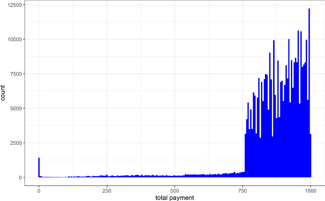
Figure A1.
Histogram of total payments below PLN 1,000 for the period 2014–2021
Table A1.
Number of beneficiaries of CAP payments by year and type (for total payments of not less than PLN 750)
| Year | Individual farmers | Small farmers | Institutional farmers | All beneficiaries | % Institutional | % Institutional in the value of total payments |
|---|---|---|---|---|---|---|
| 2014 | 1,411,568 | – | 15,223 | 1,426,791 | 1.1% | 23.8% |
| 2015 | 1,416,227 | – | 17,863 | 1,434,090 | 1.2% | 25.3% |
| 2016 | 642,091 | 745,924 | 10,039 | 1,398,054 | 0.7% | 20.5% |
| 2017 | 678,342 | 698,073 | 12,082 | 1,388,497 | 0.9% | 10.6% |
| 2018 | 679,864 | 655,660 | 8,887 | 1,344,411 | 0.7% | 13.9% |
| 2019 | 705,701 | 619,315 | 10,150 | 1,335,166 | 0.8% | 17.2% |
| 2020 | 727,453 | 573,771 | 9,324 | 1,310,548 | 0.7% | 13.4% |
| 2021 | 750,524 | 541,825 | 9,214 | 1,301,563 | 0.7% | 11.7% |
[i] Source: Own elaboration based on data published by the Ministry of Agriculture and Rural Development on https://beneficjenciwpr.minrol.gov.pl/ Note: Beneficiaries who had total payments below PLN 750 or for whom postal code information was missing are not included here. ‘Individual farmers’ are those farmers who were listed by name in the database. ‘Small farmers’ denotes farmers who joined the Small Farmers Scheme (in place since 2016). ‘Institutional farmers’ denotes all beneficiaries for whom the database does not report first name and surname and who are not listed as beneficiaries of SFS payments. The last column presents the percentage of payments that go to institutional beneficiaries. The share is calculated in total payments – namely all types of payments that are reported by the Ministry of Agriculture and Rural Development.
Table A2.
Average and median total payments and single area payments by year and type of beneficiary (for total payments of not less than PLN 750; rural municipalities only)
| Type | Year | Average total payment (PLN) | Median total payment (PLN) | % Receiving single area payments | Average single area payment (PLN) | Median single area payment (PLN) |
|---|---|---|---|---|---|---|
| Individual farmers | 2014 | 12,564.37 | 5,876.29 | 94% | 8,068.39 | 4,408.89 |
| 2015 | 14,438.64 | 6,275.89 | 94% | 8,924.12 | 4,800.28 | |
| 2016 | 23,111.17 | 13,703.34 | 92% | 14,307.21 | 9,582.33 | |
| 2017 | 20,953.64 | 12,881.24 | 94% | 13,895.78 | 9,275.02 | |
| 2018 | 22,772.81 | 12,876.52 | 97% | 13,579.06 | 8,951.87 | |
| 2019 | 22,434.67 | 12,292.40 | 98% | 13,365.31 | 8,705.32 | |
| 2020 | 24,521.88 | 12,524.77 | 98% | 13,526.19 | 8,680.80 | |
| 2021 | 26,834.20 | 13,106.54 | 97% | 13,420.43 | 8,574.87 | |
| Small farmers | 2016 | 3,176.42 | 2,576.78 | 100% | 2,495.97 | 2,206.84 |
| 2017 | 3,000.12 | 2,599.94 | 100% | 2,528.20 | 2,231.51 | |
| 2018 | 3,156.97 | 2,558.08 | 100% | 2,491.52 | 2,190.55 | |
| 2019 | 3,073.93 | 2,510.09 | 100% | 2,451.04 | 2,148.63 | |
| 2020 | 3,336.57 | 2,601.71 | 100% | 2,493.17 | 2,183.26 | |
| 2021 | 3,503.80 | 2,610.95 | 100% | 2,505.27 | 2,192.02 | |
| Institutional farmers | 2014 | 358,385.50 | 50,661.73 | 45% | 156,280.51 | 13,279.74 |
| 2015 | 376,394.86 | 71,793.19 | 42% | 156,111.07 | 12,614.01 | |
| 2016 | 419,455.13 | 148,748.05 | 53% | 176,139.70 | 56,568.09 | |
| 2017 | 144,829.82 | 18,519.16 | 40% | 171,014.03 | 51,770.90 | |
| 2018 | 333,602.93 | 108,638.00 | 63% | 164,682.63 | 44,243.18 | |
| 2019 | 381,143.53 | 124,063.96 | 54% | 161,612.76 | 41,823.51 | |
| 2020 | 349,188.61 | 116,636.81 | 60% | 160,903.89 | 39,930.64 | |
| 2021 | 297,782.05 | 100,000.00 | 63% | 156,739.69 | 37,465.25 |
[i] Note: In 2014 and 2015, ‘individual farmers’ include ‘small farmers’, who have been a separate category since 2016. For ‘small farmers’, the one-off payment was assumed to correspond to the single area payment. Beneficiaries who had total payments below PLN 750, or for whom postal code information was missing, are not included here. For ‘institutional beneficiaries’, the data for 2016/2017 should be treated with caution as it clearly departs from the rest with no obvious reason as to the case
Table A3.
TERYT codes of pairs of neighbouring urban/rural municipalities with the same name
| Municipality | Urban | Rural |
|---|---|---|
| Aleksandrów Kujawski | 0401011 | 0401042 |
| Augustów | 2001011 | 2001022 |
| Bartoszyce | 2801011 | 2801032 |
| Bełchatów | 1001011 | 1001022 |
| Biała Podlaska | 0661011 | 0601032 |
| Białogard | 3201011 | 3201022 |
| Bielsk Podlaski | 2003011 | 2003032 |
| Biłgoraj | 0602011 | 0602032 |
| Bochnia | 1201011 | 1201022 |
| Bolesławiec | 0201011 | 0201022 |
| Braniewo | 2802011 | 2802022 |
| Brańsk | 2003021 | 2003052 |
| Brodnica | 0402011 | 0402032 |
| Brzeziny | 1021011 | 1021022 |
| Chełm | 0662011 | 0603032 |
| Chełmno | 0404011 | 0404022 |
| Chełmża | 0415011 | 0415022 |
| Chodzież | 3001011 | 3001032 |
| Chojnice | 2202011 | 2202032 |
| Chojnów | 0209011 | 0209022 |
| Ciechanów | 1402011 | 1402022 |
| Czarnków | 3002011 | 3002022 |
| Człuchów | 2203011 | 2203032 |
| Darłowo | 3213011 | 3213032 |
| Dębica | 1803011 | 1803042 |
| Dynów | 1816011 | 1816052 |
| Działdowo | 2803011 | 2803022 |
| Dzierżoniów | 0202021 | 0202052 |
| Elbląg | 2861011 | 2804012 |
| Ełk | 2805011 | 2805022 |
| Garwolin | 1403011 | 1403042 |
| Giżycko | 2806011 | 2806042 |
| Głogów | 0203011 | 0203022 |
| Głowno | 1020011 | 1020052 |
| Gniezno | 3003011 | 3003032 |
| Golub-Dobrzyń | 0405011 | 0405032 |
| Gorlice | 1205011 | 1205042 |
| Gostynin | 1404011 | 1404022 |
| Górowo Iławeckie | 2801021 | 2801052 |
| Grajewo | 2004011 | 2004022 |
| Grudziądz | 0462011 | 0406012 |
| Grybów | 1210011 | 1210042 |
| Gubin | 0802011 | 802052 |
| Hajnówka | 2005011 | 2005062 |
| Hrubieszów | 0604011 | 0604042 |
| Iława | 2807011 | 2807032 |
| Inowrocław | 0407011 | 0407042 |
| Jarosław | 1804011 | 1804042 |
| Jasło | 1805011 | 1805042 |
| Jordanów | 1215011 | 1215052 |
| Kamienna Góra | 0207011 | 0207022 |
| Kętrzyn | 2808011 | 2808032 |
| Kłodzko | 0208021 | 0208072 |
| Kolno | 2006011 | 2006032 |
| Koło | 3009011 | 3009072 |
| Kołobrzeg | 3208011 | 3208042 |
| Kościan | 3011011 | 3011032 |
| Kościerzyna | 2206011 | 2206042 |
| Kowal | 0418011 | 0418092 |
| Krasnystaw | 0606011 | 0606052 |
| Kraśnik | 0607011 | 0607052 |
| Kutno | 1002011 | 1002062 |
| Kwidzyn | 2207011 | 2207032 |
| Leżajsk | 1808011 | 1808042 |
| Lidzbark Warmiński | 2809011 | 2809032 |
| Limanowa | 1207011 | 1207072 |
| Lipno | 0408011 | 0408062 |
| Lubaczów | 1809011 | 1809042 |
| Lubań | 0210011 | 0210042 |
| Lubartów | 0608011 | 0608072 |
| Lubawa | 2807021 | 2807052 |
| Lubin | 0211011 | 0211022 |
| Łańcut | 1810011 | 1810042 |
| Łaskarzew | 1403021 | 1403062 |
| Łęczyca | 1004011 | 1004052 |
| Łomża | 2062011 | 2007022 |
| Łowicz | 1005011 | 1005072 |
| Łuków | 0611011 | 0611052 |
| Malbork | 2209011 | 2209042 |
| Mielec | 1811011 | 1811052 |
| Międzyrzec Podlaski | 0601011 | 0601102 |
| Mińsk Mazowiecki | 1412011 | 1412112 |
| Mrągowo | 2810011 | 2810032 |
| Mszana Dolna | 1207021 | 1207092 |
| Nowa Ruda | 0208041 | 0208112 |
| Nowa Sól | 0804011 | 0804052 |
| Nowe Miasto Lubawskie | 2812011 | 2812052 |
| Nowy Targ | 1211011 | 1211092 |
| Obrzycko | 3024011 | 3024042 |
| Oleśnica | 0214011 | 0214062 |
| Oława | 0215011 | 0215042 |
| Ostróda | 2815011 | 2815092 |
| Ostrów Mazowiecka | 1416011 | 1416072 |
| Ostrów Wielkopolski | 3017011 | 3017042 |
| Ozorków | 1020021 | 1020062 |
| Pabianice | 1008021 | 1008072 |
| Pionki | 1425011 | 1425082 |
| Płońsk | 1420011 | 1420092 |
| Pruszcz Gdański | 2204011 | 2204042 |
| Przasnysz | 1422011 | 1422072 |
| Przemyśl | 1862011 | 1813082 |
| Przeworsk | 1814011 | 1814062 |
| Puck | 2211031 | 2211072 |
| Puławy | 0614011 | 0614092 |
| Raciąż | 1420021 | 1420102 |
| Radomsko | 1012011 | 1012122 |
| Radymno | 1804021 | 1804082 |
| Radziejów | 0411011 | 0411062 |
| Radzyń Podlaski | 0615011 | 0615062 |
| Rawa Mazowiecka | 1013011 | 1013042 |
| Słupsk/Redzikowo | 2263011 | 2212082 |
| Rejowiec Fabryczny | 0603011 | 0603082 |
| Rypin | 0412011 | 0412042 |
| Sanok | 1817011 | 1817052 |
| Sejny | 2009011 | 2009052 |
| Siedlce | 1464011 | 1426082 |
| Siemiatycze | 2010011 | 2010092 |
| Sieradz | 1014011 | 1014082 |
| Sierpc | 1427011 | 1427052 |
| Skierniewice | 1063011 | 1015082 |
| Skórcz | 2213021 | 2213102 |
| Sławno | 3213021 | 1007072 |
| Słupca | 3023011 | 3023062 |
| Sochaczew | 1428011 | 1428072 |
| Sokołów Podlaski | 1429011 | 1429082 |
| Stargard | 3214011 | 3214102 |
| Starogard Gdański | 2213031 | 2213122 |
| Stoczek Łukowski | 0611021 | 0611082 |
| Suwałki | 2063011 | 2012072 |
| Szczecinek | 3215011 | 3215062 |
| Szczytno | 2817011 | 2817062 |
| Świdnica | 219011 | 219072 |
| Świdwin | 3216011 | 3216062 |
| Tarnów | 1263011 | 1216092 |
| Tczew | 2214011 | 2214062 |
| Terespol | 0601021 | 0601162 |
| Tomaszów Lubelski | 0618011 | 0618112 |
| Tomaszów Mazowiecki | 1016011 | 1016092 |
| Turek | 3027011 | 3027082 |
| Ustka | 2212011 | 2212102 |
| Wałcz | 3217011 | 3217052 |
| Wąbrzeźno/Ryńsk | 0417011 | 0417052 |
| Wągrowiec | 3028011 | 3028072 |
| Wejherowo | 2215031 | 2215102 |
| Włocławek | 0464011 | 0418132 |
| Włodawa | 0619011 | 0619062 |
| Wysokie Mazowieckie | 2013011 | 2013102 |
| Zambrów | 2014011 | 2014052 |
| Zamość | 0664011 | 0620142 |
| Zduńska Wola | 1019011 | 1019042 |
| Zgierz | 1020031 | 1020092 |
| Zgorzelec | 0225021 | 0225072 |
| Złotoryja | 0226021 | 0226062 |
| Złotów | 3031011 | 3031082 |
| Żagań | 0810021 | 0810092 |
| Żary | 0811021 | 0811102 |
Table 4.
Summary statistics of total payments (based on rural municipalities and individual beneficiaries with total payments of at least PLN 750) – country level
| Statistic | 2014 | 2015 | 2016 | 2017 | 2018 | 2019 | 2020 | 2021 |
|---|---|---|---|---|---|---|---|---|
| no. of obs. | 729,536 | 730,897 | 713,962 | 708,029 | 687,517 | 678,698 | 673,242 | 669,220 |
| min (PLN) | 750 | 750 | 750 | 750 | 750 | 751 | 750 | 751 |
| max (PLN) | 13.76 mln | 7.08 mln | 17.75 mln | 2.75 mln | 5.02 mln | 3.29 mln | 5.04 mln | 5.00 mln |
| mean (PLN) | 12,564 | 14,439 | 12,956 | 12,324 | 13,624 | 13,842 | 15,585 | 17,472 |
| median (PLN) | 5,876 | 6,276 | 5,663 | 5,605 | 5,613 | 5,583 | 5,900 | 6,117 |
| Theil | 0.828 | 0.912 | 0.830 | 0.756 | 0.855 | 0.883 | 0.912 | 0.932 |
| Gini | 0.612 | 0.637 | 0.627 | 0.612 | 0.639 | 0.645 | 0.660 | 0.671 |
| Atkinson | 0.502 | 0.532 | 0.527 | 0.507 | 0.543 | 0.551 | 0.572 | 0.592 |
| sd of log | 1.083 | 1.104 | 1.147 | 1.131 | 1.173 | 1.180 | 1.213 | 1.260 |
| q90/10 | 16.857 | 16.072 | 20.109 | 19.849 | 22.148 | 22.538 | 24.767 | 28.670 |
| q95/05 | 29.683 | 34.407 | 39.613 | 38.109 | 42.918 | 43.689 | 47.812 | 52.668 |
| q75/25 | 4.784 | 4.628 | 5.444 | 5.401 | 5.635 | 5.710 | 5.918 | 6.556 |
| q99/01 | 135.849 | 152.757 | 128.961 | 111.724 | 135.814 | 141.373 | 172.507 | 190.820 |
| q90/50 | 4.454 | 4.303 | 5.035 | 5.059 | 5.600 | 5.693 | 6.183 | 7.032 |
| q50/10 | 3.785 | 3.736 | 3.994 | 3.924 | 3.955 | 3.959 | 4.005 | 4.077 |
| share top 1% | 17.8% | 18.5% | 15.8% | 14.0% | 16.5% | 17.2% | 16.6% | 16.1% |
| share top 10% | 49.6% | 53.3% | 49.8% | 47.7% | 50.7% | 51.4% | 53.2% | 53.5% |
| share bottom 1% | 0.1% | 0.1% | 0.1% | 0.1% | 0.1% | 0.1% | 0.1% | 0.0% |
| share bottom 10% | 1.0% | 0.9% | 0.9% | 0.9% | 0.8% | 0.8% | 0.7% | 0.7% |
[i] Note: Own elaboration. All the measures were calculated at country level – that is, for all beneficiaries taken together. Only rural municipalities and individual farmers with total payments of not less than PLN 750 are included. Variables denoted as ‘qX/Y’ refer to different percentile ratios as indicated by X and Y
Table A5.
Gini of total payments by year and voivodeship (based on rural municipalities and individual beneficiaries with total payments of at least PLN 750)
| Voivodeship | Year | |||||||
|---|---|---|---|---|---|---|---|---|
| 2014 | 2015 | 2016 | 2017 | 2018 | 2019 | 2020 | 2021 | |
| Poland | 0.612 | 0.637 | 0.627 | 0.612 | 0.639 | 0.645 | 0.660 | 0.671 |
| Dolnośląskie | 0.681 | 0.684 | 0.678 | 0.686 | 0.706 | 0.709 | 0.713 | 0.719 |
| Kujawsko-pomorskie | 0.583 | 0.611 | 0.586 | 0.580 | 0.605 | 0.610 | 0.617 | 0.628 |
| Lubelskie | 0.577 | 0.611 | 0.583 | 0.575 | 0.616 | 0.620 | 0.648 | 0.652 |
| Lubuskie | 0.724 | 0.743 | 0.721 | 0.714 | 0.722 | 0.726 | 0.722 | 0.723 |
| Łódzkie | 0.535 | 0.584 | 0.545 | 0.539 | 0.583 | 0.581 | 0.604 | 0.615 |
| Małopolskie | 0.565 | 0.608 | 0.568 | 0.544 | 0.606 | 0.602 | 0.633 | 0.658 |
| Mazowieckie | 0.565 | 0.581 | 0.570 | 0.536 | 0.559 | 0.582 | 0.595 | 0.618 |
| Opolskie | 0.663 | 0.693 | 0.672 | 0.660 | 0.684 | 0.682 | 0.687 | 0.705 |
| Podkarpackie | 0.625 | 0.609 | 0.596 | 0.595 | 0.630 | 0.624 | 0.652 | 0.669 |
| Podlaskie | 0.477 | 0.513 | 0.492 | 0.514 | 0.534 | 0.529 | 0.554 | 0.566 |
| Pomorskie | 0.618 | 0.662 | 0.630 | 0.611 | 0.629 | 0.640 | 0.644 | 0.648 |
| Śląskie | 0.661 | 0.682 | 0.651 | 0.645 | 0.684 | 0.670 | 0.694 | 0.695 |
| Świętokrzyskie | 0.577 | 0.598 | 0.628 | 0.536 | 0.605 | 0.589 | 0.633 | 0.637 |
| Warmińsko-mazurskie | 0.595 | 0.601 | 0.588 | 0.598 | 0.606 | 0.609 | 0.621 | 0.619 |
| Wielkopolskie | 0.594 | 0.638 | 0.634 | 0.589 | 0.604 | 0.626 | 0.641 | 0.653 |
| Zachodniopomorskie | 0.682 | 0.710 | 0.684 | 0.672 | 0.684 | 0.686 | 0.701 | 0.705 |
Table A6.
The biggest changes in the Gini coefficient between 2014 and 2021 in rural municipalities, based on direct payments to non-institutional beneficiaries (total payments > PLN 750, municipalities with > 100 beneficiaries)
| TERYT | Name of municipality | Gini 2014 | Gini 2021 | Change | |
|---|---|---|---|---|---|
| 10 largest decreases | 3020052 | Gołuchów | 0.813 | 0.652 | −0.161 |
| 2417062 | Lipowa | 0.601 | 0.475 | −0.126 | |
| 1406032 | Chynów | 0.753 | 0.630 | −0.123 | |
| 1417072 | Sobienie-Jeziory | 0.759 | 0.640 | −0.119 | |
| 1215082 | Zawoja | 0.583 | 0.468 | −0.116 | |
| 1403132 | Wilga | 0.750 | 0.661 | −0.089 | |
| 1418052 | Prażmów | 0.719 | 0.631 | −0.088 | |
| 3026012 | Brodnica | 0.658 | 0.571 | −0.087 | |
| 2404072 | Konopiska | 0.782 | 0.695 | −0.087 | |
| 2604172 | Sitkówka-Nowiny | 0.608 | 0.522 | −0.087 | |
| 10 largest increases | 1425072 | Kowala | 0.549 | 0.832 | 0.283 |
| 1207062 | Laskowa | 0.388 | 0.636 | 0.248 | |
| 1201042 | Lipnica Murowana | 0.486 | 0.726 | 0.240 | |
| 1005032 | Chąśno | 0.411 | 0.643 | 0.232 | |
| 2611022 | Brody | 0.452 | 0.681 | 0.230 | |
| 1209052 | Raciechowice | 0.451 | 0.662 | 0.211 | |
| 2417132 | Świnna | 0.467 | 0.676 | 0.209 | |
| 1206042 | Jerzmanowice-Przeginia | 0.449 | 0.657 | 0.208 | |
| 2601052 | Solec-Zdrój | 0.514 | 0.715 | 0.202 | |
| 1816072 | Hyżne | 0.447 | 0.641 | 0.194 |
[i] Note: Own elaboration. Gini coefficients were calculated at municipality level. Only rural municipalities with at least 100 beneficiaries are included. In addition, only individual farmers with total payments no less than PLN 750 are considered. TERYT is a unique identifier of units of territorial division in Poland