
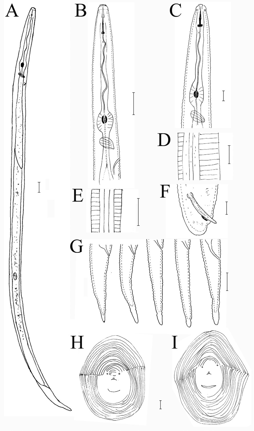
Figure 1
Meloidogyne paramali n. sp. A: J2; B: Anterior region of J2; C: Anterior region of male; D: Lateral region of male; E: Lateral region of J2; F: Male tail region; G: Variations of J2 tail; H, I: Female perineal patterns. (Scale bars = 10 μm).
Table 1
Morphometrics of J2 of Meloidogyne paramali n. sp and M. mali. All measurements are in micrometer and in the form: mean ± s.d. (range).
| Meloidogyne paramali n. sp | M. mali detected from Japanese maple treea | ||
|---|---|---|---|
| Holotype J2 | Paratype J2s | - | |
| n | 20 | 20 | |
| Body length | 441 | 433 ± 13.1 (402–455) | 425 ± 30.1 (362–466) |
| Body width | 14.2 | 13.7 ± 0.8 (12.5–15.3) | 14.0 ± 1.1 (13.1–18.1) |
| Head end to metacorpus valve | 60.2 | 58.6 ± 2.2 (54–64) | 53.5 ± 2.1 (49.5–56.8) |
| Head end to excretory pore | 80.6 | 76.4 ± 3.6 (64–80.8) | 74.1 ± 4.2 (68.8–82.3) |
| Head width | 5.7 | 5.6 ± 0.2 (5.0–5.9) | 5.1 ± 0.41 (4.1–5.7) |
| Head height | 3.2 | 3.0 ± 0.3 (2.2–3.5) | 2.6 ± 0.32 (2.1–3.2) |
| Stylet length | 11.8 | 11.7 ± 0.5 (10.8–12.5) | 10.5 ± 0.5 (9.5–11.6) |
| Stylet conus | 6.5 | 6.4 ± 0.3 (6.0–7.0) | 5.7 ± 0.5 (4.7–6.7) |
| Knobs height | 1.1 | 1.1 ± 0.1 (0.9–1.2) | 1.2 ± 0.2 (0.8–1.6) |
| Knobs width | 2.0 | 1.8 ± 0.3 (1.5–2.4) | 2.1 ± 0.2 (1.8–2.7) |
| DGO | 3.6 | 3.3 ± 0.3 (2.4–3.9) | 4.4 ± 0.57 (3.5–5.5) |
| Tail length | 33.6 | 32.2 ± 3.5 (24–36.8) | 32.7 ± 3.0 (29.2–39.3) |
| Anal body diam. | 8.2 | 8.0 ± 0.6 (6.9–8.7) | 7.9 ± 0.9 (5.9–9.6) |
| Tail hyaline portion | 4.3 | 4.3 ± 0.6 (3.0–4.9) | 7.2 ± 2.3 (3.9–9.3) |
| a | 31.0 | 31.7 ± 1.6 (28.2–34.8) | 30.4 ± 2.6 (25.2–34.5) |
| b(body length/Head end to metacorpus valve) | 7.3 | 7.4 ± 0.2 (7.0–7.7) | 8.0 ± 0.6 (6.8–9.2) |
| c | 13.1 | 13.6 ± 1.9 (11.7–18.9) | 13.2 ± 1.1 (11.6–15.3) |
| c’ | 4.1 | 4.1 ± 0.5 (2.8–4.8) | 4.2 ± 0.7 (3.1–5.6) |
| m | 55.0 | 54.1 ± 2.9 (50.5–58.9) | 54.5 ± 3.8 (47–60.3) |
| O | 30.5 | 28.1 ± 3.7 (21.4–34.5) | 41.9 ± 5.8 (31.6–53.9) |
| Head width/head height | 1.8 | 1.87 ± 0.2 (1.7–2.5) | 2.0 ± 0.2 (1.6–2.3) |
| h% (Tail hyaline portion/tail length×100) | 12.8 | 13.7 ± 1.8 (9.8–17.1) | 21.7 ± 5.9 (12.7–27.8) |
[i] aGu et al., 2013.
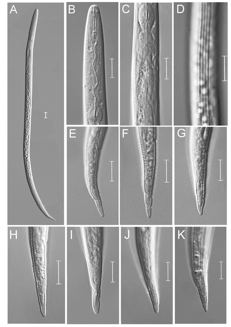
Figure 2
Light photomicrographs of Meloidogyne paramali n. sp. J2. A: Entire body; B: Anterior region; C: Post median bulb region; D: Lateral region; E–K: Tail region. (Scale bars = 10 μm).
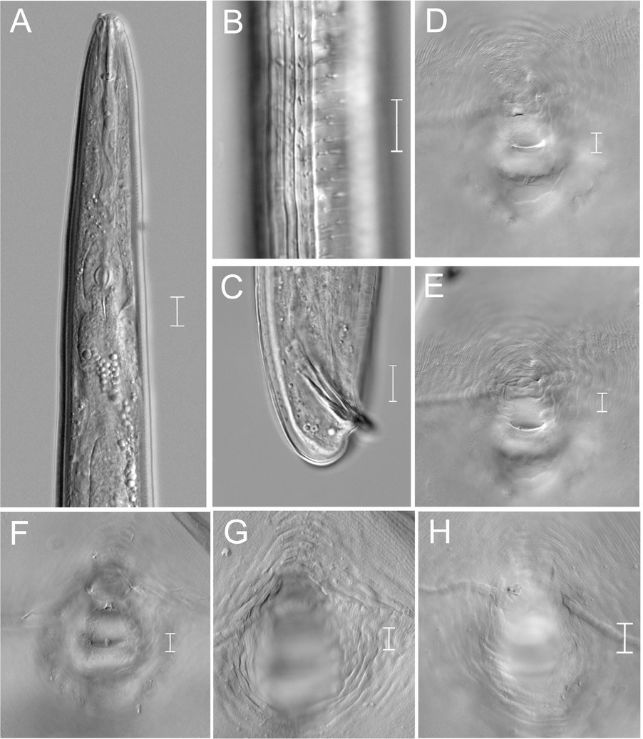
Figure 3
Light photomicrographs of Meloidogyne paramali n. sp. male and female. A: Male head region; B: Male lateral region; C: Male tail region; D–H: Female perineal patterns. (Scale bars = 10 μm).
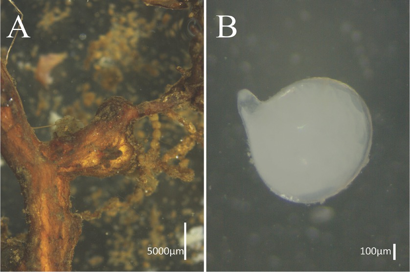
Figure 4
Light photomicrographs of host plant roots infected by Meloidogyne paramali n. sp. and female. A: Root-knot; B: Female.
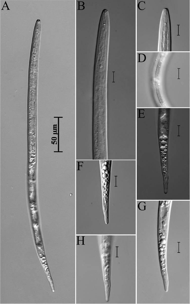
Figure 5
Light photomicrographs of Meloidogyne marylandi J2. A: Entire body; B, C: Anterior region; D: Lateral region; E–H: Tail region. (Scale bars = 10 μm).
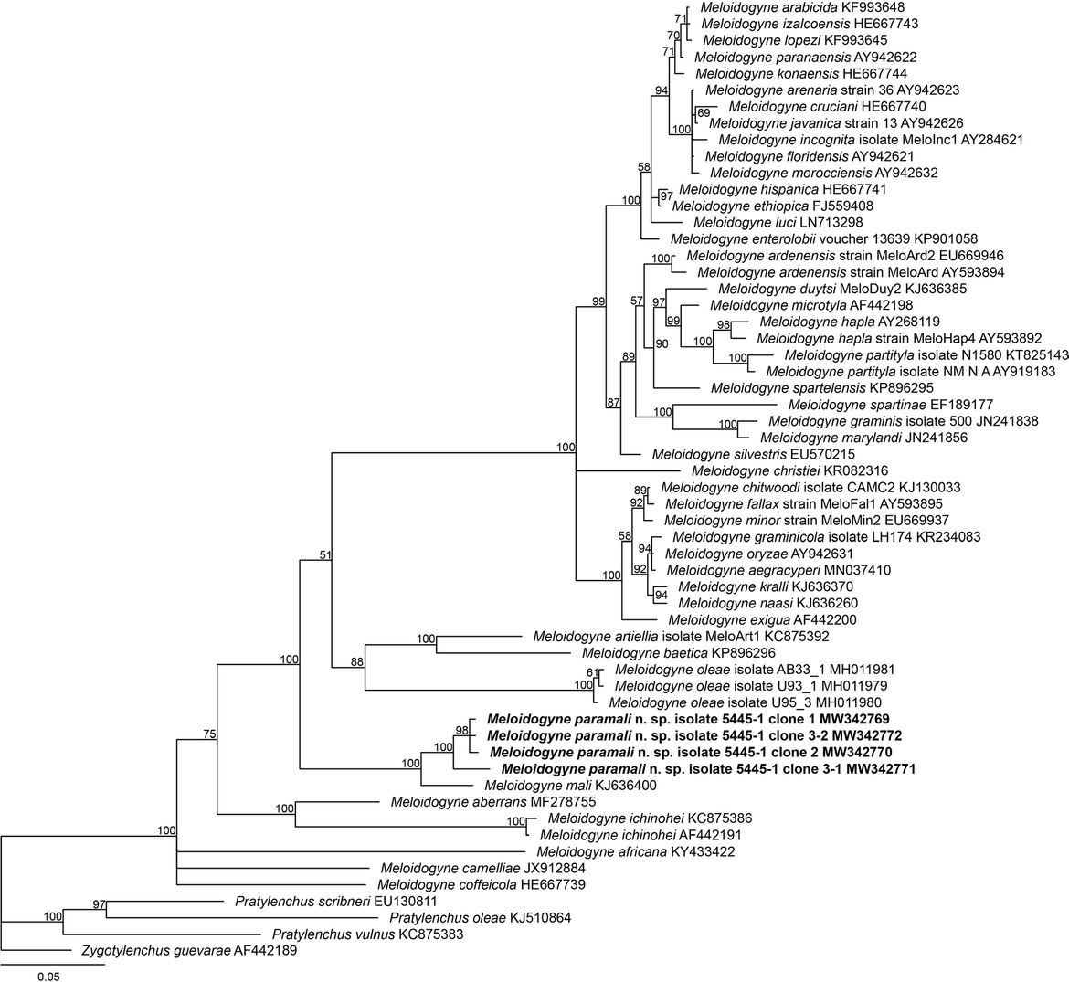
Figure 6
Phylogenetic relationships of the Melodidogyne paramali n. sp. within the genus Meloidogyne as inferred from Bayesian analysis of the 18S rDNA sequences using the SYM + I + G model (ln L = −9,656.5775; freqA = 0.2500; freqC = 0.2500; freqG = 0.2500; freqT = 0.2500; R(a) = 1.1490; R(b) = 2.9493; R(c) = 1.9703; R(d) = 0.5777; R(e) = 4.7703; R(f) = 1.0000; Pinva = 0.4140; Shape = 0.4400). Posterior probabilities are given in clades node. Newly obtained sequences are indicated in bold and the sequence codes are given in specimen-clone.
Table 2
Morphometrics of J2 of Meloidogyne marylandi and other populations. All measurements are in micrometer and in the form: mean ± s.d. (range).
| Japan on Podocarpus macrophyllus | Japan on Panicum crus-gallia | Israel on Avena strigosab | USA on Zoysia japonicac | |
|---|---|---|---|---|
| n | 14 | 100 | - | 20 |
| L | 381.7 ± 20.7 | 392.3 ± 22.05 | 442.9 ± 13.5 | 395.1 ± 12.5 |
| (351.7–418.4) | (338.6–449.3) | (396.0–445.5) | (367.8–411.8) | |
| Body width | 13.9 ± 0.6 | 15.7 ± 0.44 | 14.8 ± 0.8 | 16.2 ± 0.8 |
| (12.8–14.7) | (14.2–16.6) | (13.4–15.9) | (14.8–17.7) | |
| Stylet length | 12.5 ± 0.6 | 12.9 ± 0.45 | 11.0 ± 0.4 | 10.8 ± 0.3 |
| (11.5–13.4) | (11.5–14.1) | (10.4–11.9) | (10.6–11.2) | |
| Stylet base to head | 14.5 ± 0.4 (13.7–15.0) | 15.4 ± 0.46 (13.7–16.6) | 14.6 ± 0.7 (13.4–15.9) | – – |
| DGO | 3.1 ± 0.3 | 2.5 ± 0.26 | 2.6 ± 0.4 | 2.4 ± 0.1 |
| (2.8–3.6) | (1.8–3.1) | (2.2–2.9) | (1.8–2.9) | |
| Head end to metacorpus valve | 55.3 ± 2.4 (51.0–57.9) | 45.7 ± 7.3 (30.1–66.3) | 52.8 ± 1.9 (51.2–54.9) | 51.3 ± 1.4 (49.5–54.3) |
| Tail length | 52.7 ± 1.5 | 63.7 ± 2.73 | 63.1 ± 3.1 | 57.9 ± 1.6 |
| (49.5–54.0) | (53.6–70.5) | (60.4–69.3) | (55.5–60.2) | |
| Tail hyaline portion | 11.2 ± 1.2 (9.5–13.5) | 12.3 ± 1.1 (9.3–14.7) | 12.4 ± 0.9 (9.9–13.4) | 11.5 ± 0.6 (10.0–12.4) |
| a | 27.4 ± 1.2 | 25.0 ± 1.3 | 28.8 ± 1.7 | 24.5 ± 1.0 |
| (26.4–30.2) | (22.3–28.4) | (26.2–31.3) | (22.9–26.4) | |
| c | 7.2 ± 0.3 | 6.2 ± 0.29 | 6.8 ± 0.4 | 6.8 ± 0.2 |
| (7.0–7.9) | (5.5–7.1) | (6.3–7.6) | (6.4–7.3) |
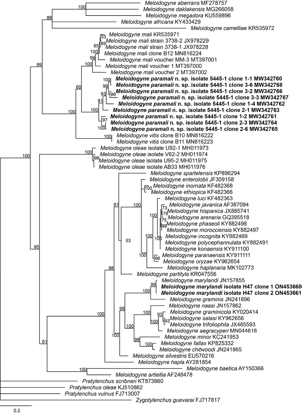
Figure 7
Phylogenetic relationships of the Melodidogyne paramali n. sp. within the genus Meloidogyne as inferred from Bayesian analysis of the ITS region of rDNA sequences using the GTR+ G model (ln L = –15,611.9209; freqA = 0.2778; freqC = 0.1784; freqG = 0.2084; freqT = 0.3354; R(a) = 1.1160; R(b) = 2.3301; R(c) = 1.4759; R(d) = 0.7128; R(e) = 2.9133; R(f) = 1.0000; Shape = 0.5730). Posterior probabilities are given in clades node. Newly obtained sequences are indicated in bold and the sequence codes are given in specimen-clone.
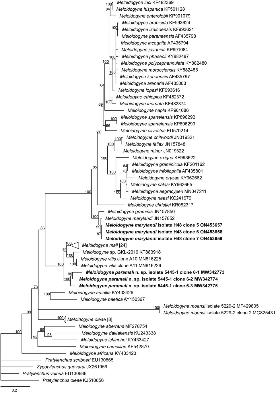
Figure 8
Phylogenetic relationships of the Melodidogyne paramali n. sp. within the genus Meloidogyne as inferred from Bayesian analysis of the D2–D3 region of the 28S rDNA sequences using the TVM + I + G model (ln L = –9,976.1624; freqA = 0.2157; freqC = 0.1943; freqG = 0.2737; freqT = 0.3163; R(a) = 1.1061; R(b) = 3.8613; R(c) = 1.8155; R(d) = 0.4745; R(e) = 3.8613; R(f) = 1.0000; Pinva = 0.2180; Shape = 0.7340). Posterior probabilities are given in clades node. Newly obtained sequences are indicated in bold and the sequence codes are given in specimen-clone.
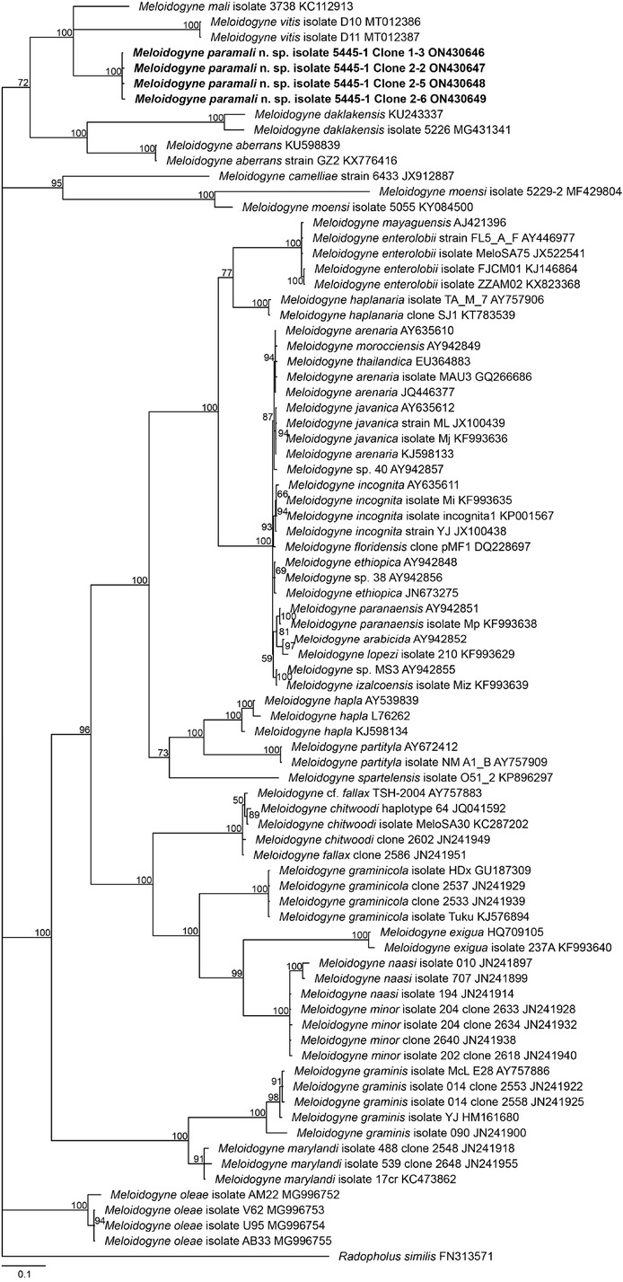
Figure 9
Phylogenetic relationships of the Melodidogyne paramali n. sp. within the genus Meloidogyne as inferred from Bayesian analysis of the intergenic region between CO II and 16S rDNA sequences using the GTR + G model (ln L = −9,869.8599; freqA = 0.3676; freqC = 0.0265; freqG = 0.0939; freqT = 0.5121; R(a) = 3.2156; R(b) = 5.9094; R(c) = 1.5251; R(d) = 2.6383; R(e) = 13.9890; R(f) = 1.0000; Shape = 0.6340). Posterior probabilities are given in clades node. Newly obtained sequences are indicated in bold and the sequence codes are given in specimen-clone.