
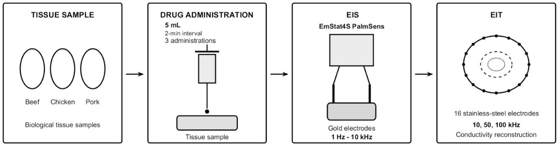
Figure 1:
Experimental workflow for monitoring drug dispersion in biological tissues using EIS and EIT.
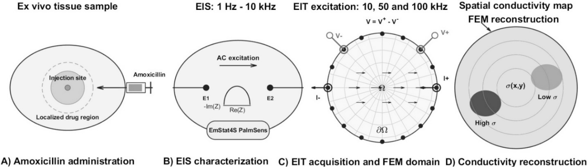
Figure 2:
Schematic diagram of A) localized dispersion near the injection site, B) analyses with EIS, C) reconstruction of the domain using FEM, D) images reconstructed of possible transport patterns that produce spatial conductivity variations detectable by EIT.
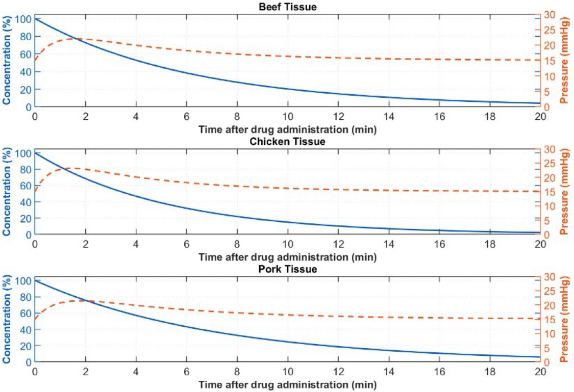
Figure 3:
Temporal evolution of fluid pressure and drug concentration for beef, chicken, and pork tissues.
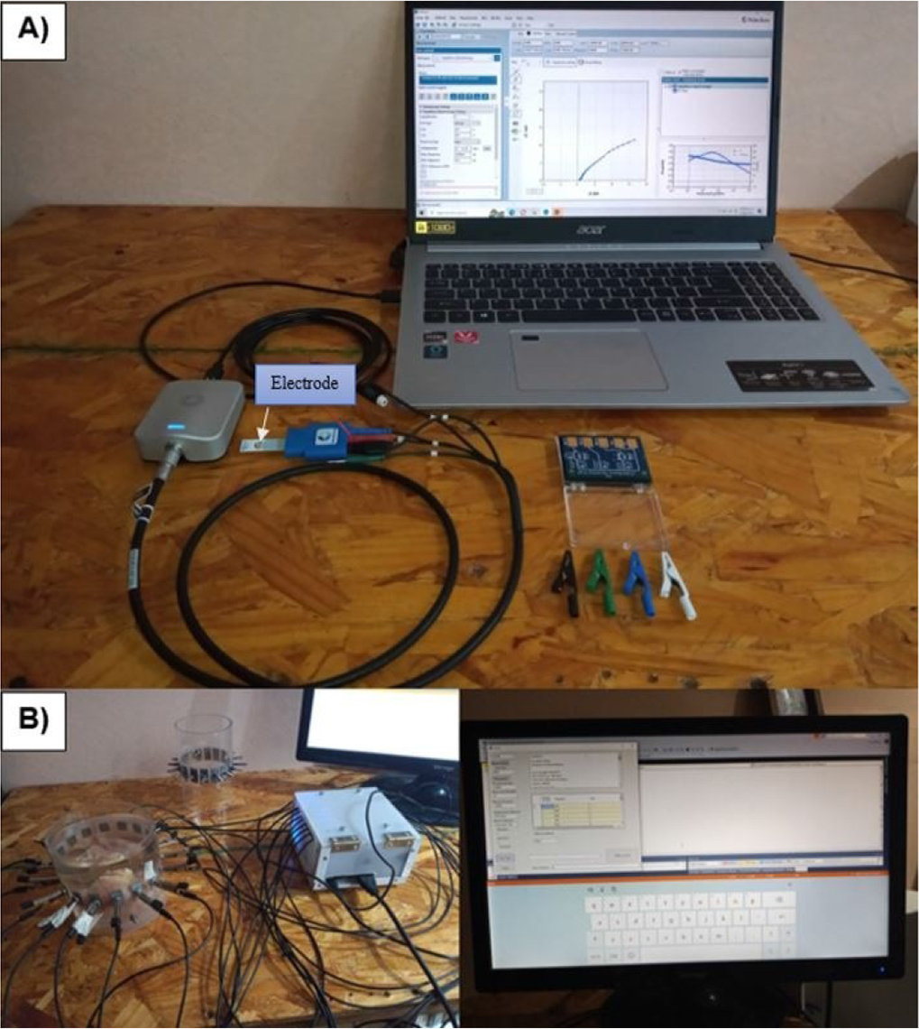
Figure 4:
Experimental setup. A) PalmSens EmStat4s®, B) SBC LattePanda Alpha® integrated to Arduino Leonardo® board.
Table 1.
Experimental parameters for EIS and EIT analysis of biological tissues.
| Parameter | Beef tissue | Chicken tissue | Pork tissue |
|---|---|---|---|
| Tissue mass | 250 g | 250 g | 250 g |
| Tissue type | Muscle | Muscle | Muscle |
| Tissue volume | 217 cm3 | 235 cm3 | 250 cm3 |
| Number of samples | 2 | 2 | 2 |
| Initial condition | Fresh | Fresh | Fresh |
| Drug | Amoxicillin | Amoxicillin | Amoxicillin |
| EIS drug volume | 0.25 mL | 0.25 mL | 0.25 mL |
| Number of administrations | 3 | 3 | 3 |
| Administration interval | 2 min | 2 min | 2 min |
| EIS Total drug volume | 1.5 mL | 1.5 mL | 1.5 mL |
| EIS frequency range | 1 Hz–10 kHz | 1 Hz–10 kHz | 1 Hz–10 kHz |
| EIS electrode | Gold | Gold | Gold |
| EIT frequencies | 10, 50, 100 kHz | 10, 50, 100 kHz | 10, 50, 100 kHz |
| EIT electrodes | 16 stainless-steel | 16 stainless-steel | 16 stainless-steel |
| EIT drug volume | 5 mL | 5 mL | 5 mL |
| EIT Total drug volume | 15 mL | 15 mL | 15 mL |
| EIT reconstruction | Conductivity distribution | Conductivity distribution | Conductivity distribution |
| Administration interval | (0, 2, 4 min) | (0, 2, 4 min) | (0, 2, 4 min) |
| Temperature | [25°C] | [25°C] | [25°C] |
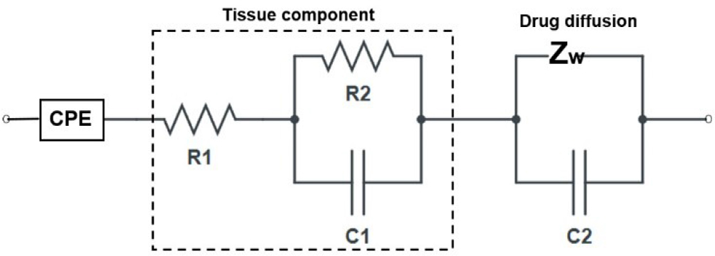
Figure 5:
Equivalent circuit model of electrode–electrolyte interface and drug diffusion in tissue [17].
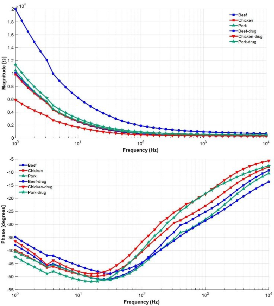
Figure 6:
Summary for drug and tissue state-space fitting model impedance data in the frequency range 1 Hz to 10 kHz.
Table 2.
Summary of the equivalent circuit model with two poles and two zeros using systems identification.
| %Fit | Beef | Chicken | Pork | Drug |
|---|---|---|---|---|
| 92.25% | 92.82% | 92.49% | 92.34% | |
| R1 (Ω) | 386.24 | 502.0 | 342.79 | 571.47 |
| R2 (Ω) | 2071.49 | 2274.92 | 1691.52 | 1984.57 |
| R3 (Ω) | 1.18×10⁴ | 1.31×10⁴ | 6.49×10³ | 1.05×10⁴ |
| C2 (F) | 3.5×10⁻⁵ | 3.6×103.5×10−5 | 3.3×103.5×10−5 | 3.3×103.5×10−5 |
| C3 (F) | 8.0×103.5×10−5 | 8.1×103.5×10−5 | 1.0×103.5×10−4 | 1.1×103.5×10−4 |
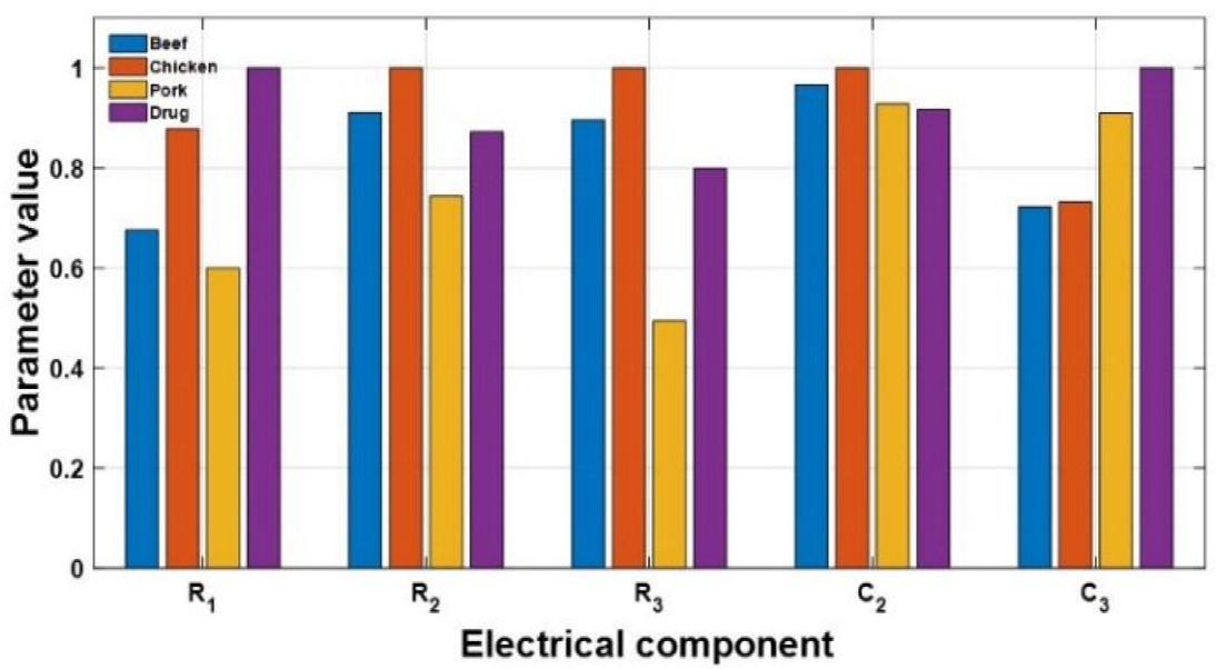
Figure 7:
Normalized Differences Between Samples.
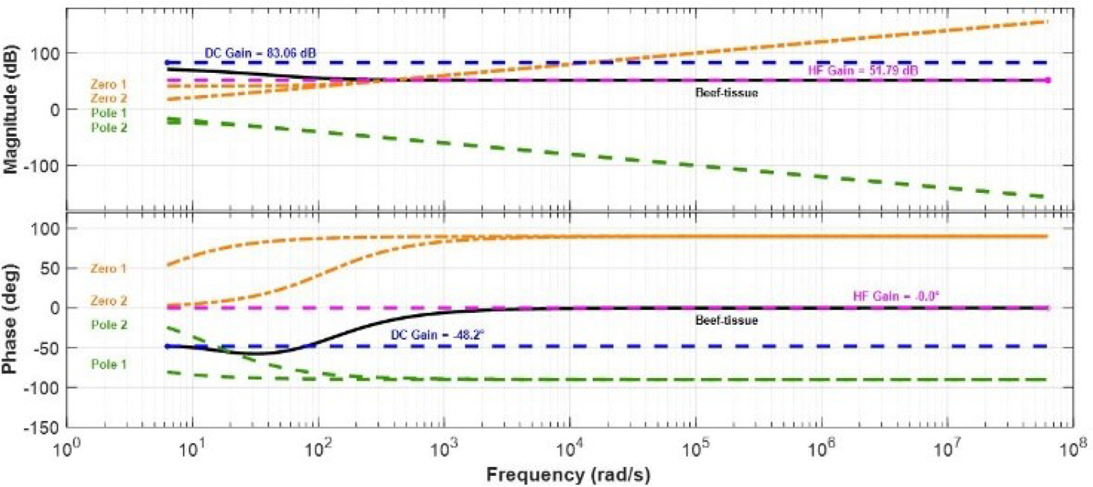
Figure 8:
Bode plot for beef tissue showing the individual contributions of each pole and zero.
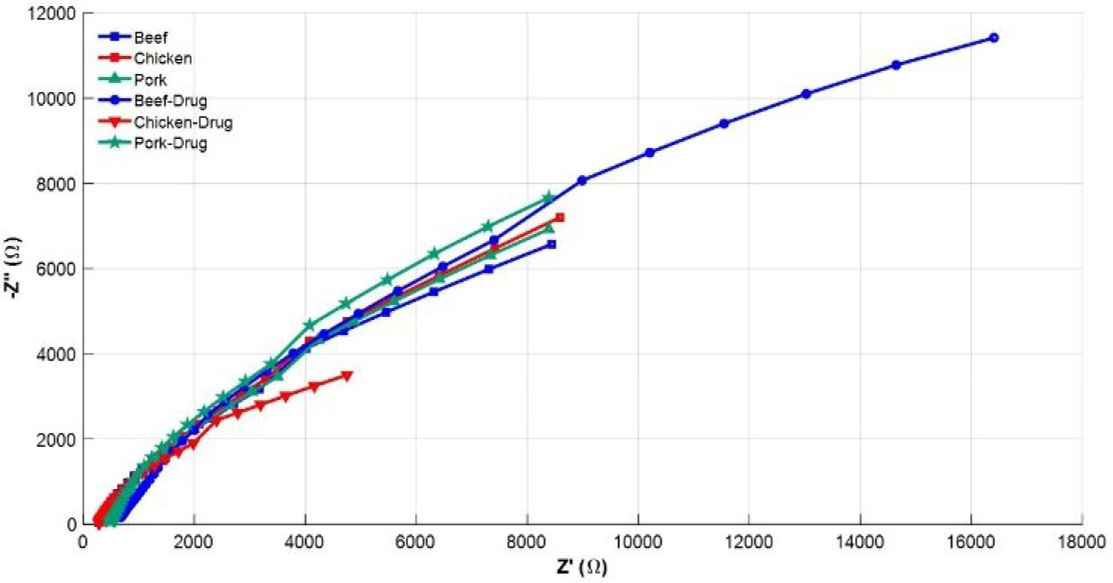
Figure 9:
Nyquist diagrams for tissues and drug.
Table 3.
Comparison between control and drug-treated tissue across the impedance spectrum.
| Tissue | Beef | Chicken | Pork |
|---|---|---|---|
| Mean control | 2027.36 | 2062.64 | 2123.25 |
| SD control | 2643.90 | 2545.45 | 2694.16 |
| Mean treated | 4622.99 | 1306.68 | 2421.41 |
| SD treated | 5369.22 | 1536.33 | 2908.57 |
| Mean difference | 2595.63 | −755.96 | 298.16 |
| Lower limit at 95% | 1730.71 | −1074.75 | 229.47 |
| Upper limit at 95% | 3460.56 | −437.16 | 366.85 |
| t-value | 6.07 | −4.79 | 8.77 |
| Degrees of freedom | 40 | 40 | 40 |
| p-value | 3.82×10⁻⁷ | 2.28×10⁻⁵ | 7.31×10⁻¹¹ |
| p-Bonferroni | 1.14×10⁻⁶ | 6.86×10⁻⁵ | 2.19×10⁻¹⁰ |
| Cohen-d | 0.93 | −0.73 | 1.34 |
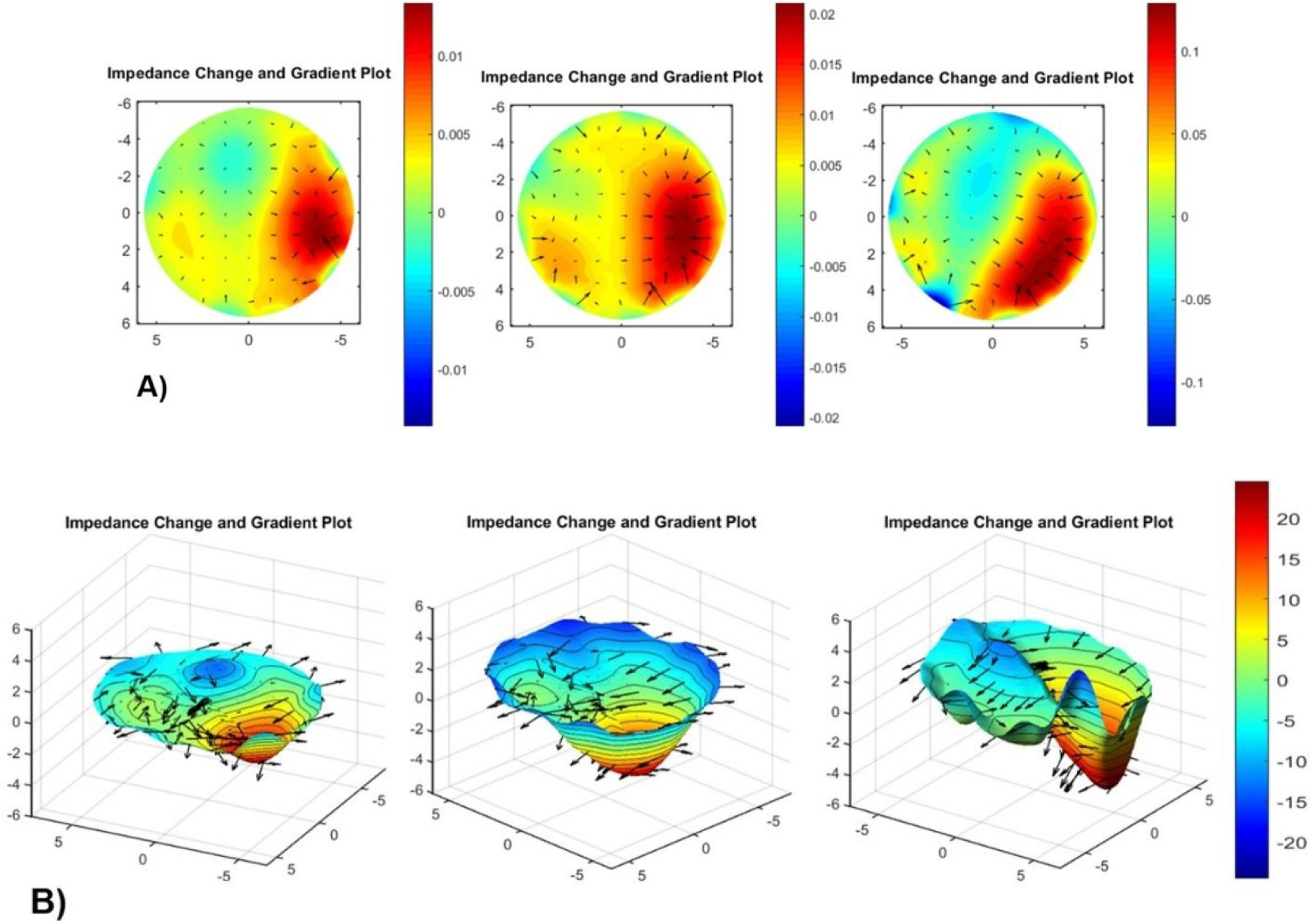
Figure 10:
Spatial conductivity changes associated with drug administration in beef tissue. A) two-dimensional and B) three-dimensional for 400 mV and 50 kHz.
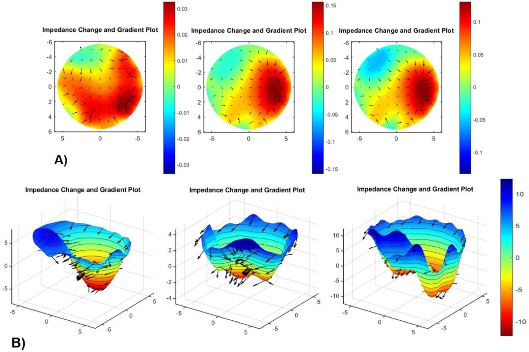
Figure 11:
Spatial conductivity changes associated with drug administration in chicken tissue. A) two-dimensional and B) three-dimensional for 400 mV and 10 kHz.
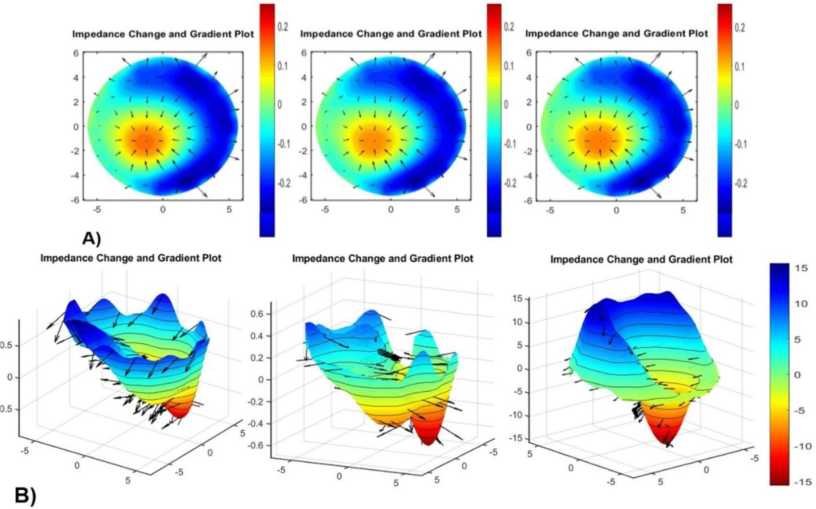
Figure 12:
Spatial conductivity changes associated with drug administration in pork tissue. A) two-dimensional and B) three-dimensional for 200 mV and 50 kHz.
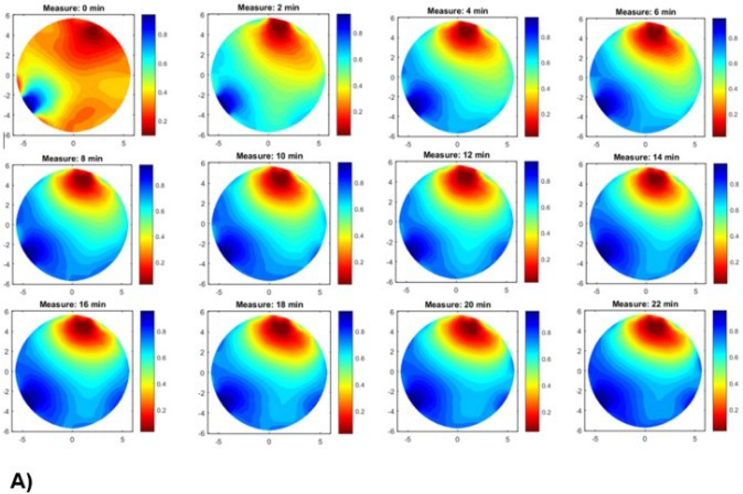
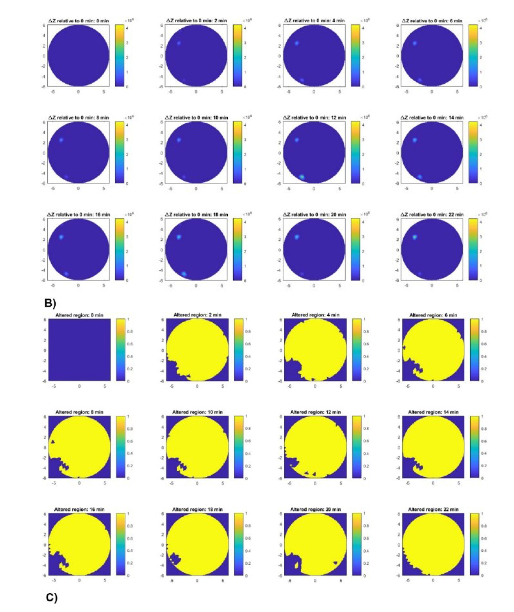
Figure 13:
A) EIT image reconstruction in beef tissue at different times. B) Spatial distribution of impedance changes relative to baseline. C) Region with impedance change.
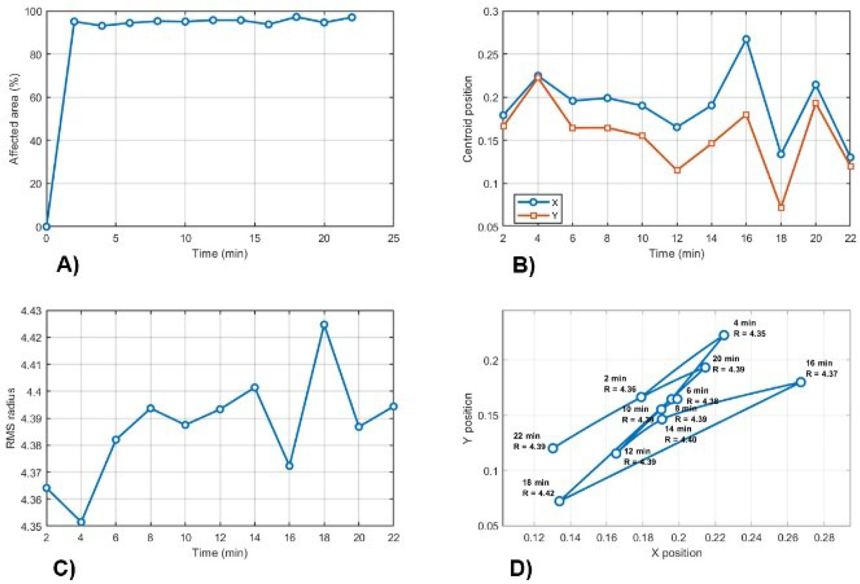
Figure 14:
Summary for A) temporal evolution of spatial extent, B) centroid movement, C) dispersion radius, and D) centroid trajectory and dispersion.
Table 4.
Summary of quantitative results.
| Time (min) | Points | Area (%) | Centroi d X | Centroi d Y | RMS |
|---|---|---|---|---|---|
| 0.0 | 0.0 | 0.0 | NaN | NaN | NaN |
| 2.0 | 441 | 95.04 | 0.179 | 0.166 | 4.36 |
| 4.0 | 432 | 93.10 | 0.225 | 0.222 | 4.35 |
| 6.0 | 438 | 94.40 | 0.196 | 0.164 | 4.38 |
| 8.0 | 442 | 95.26 | 0.199 | 0.165 | 4.39 |
| 10.0 | 441 | 95.04 | 0.190 | 0.155 | 4.38 |
| 12.0 | 444 | 95.69 | 0.165 | 0.115 | 4.39 |
| 14.0 | 444 | 95.69 | 0.191 | 0.146 | 4.40 |
| 16.0 | 435 | 93.75 | 0.267 | 0.180 | 4.37 |
| 18 | 451 | 97.20 | 0.134 | 0.072 | 4.42 |
| 20.0 | 439 | 94.61 | 0.214 | 0.193 | 4.38 |
| 22.0 | 450 | 96.98 | 0.130 | 0.120 | 4.39 |
Table 5.
Quantitative spatial resolution values for the reconstructed images.
| Tissue | FWHM (pixels) | Localization error (pixels) | Relative error (error/FWHM) |
|---|---|---|---|
| Beef | 261.57 | 156.31 | 0.59 |
| Chicken | 262.23 | 116.28 | 0.44 |
| Pork | 299.69 | 145.34 | 0.51 |
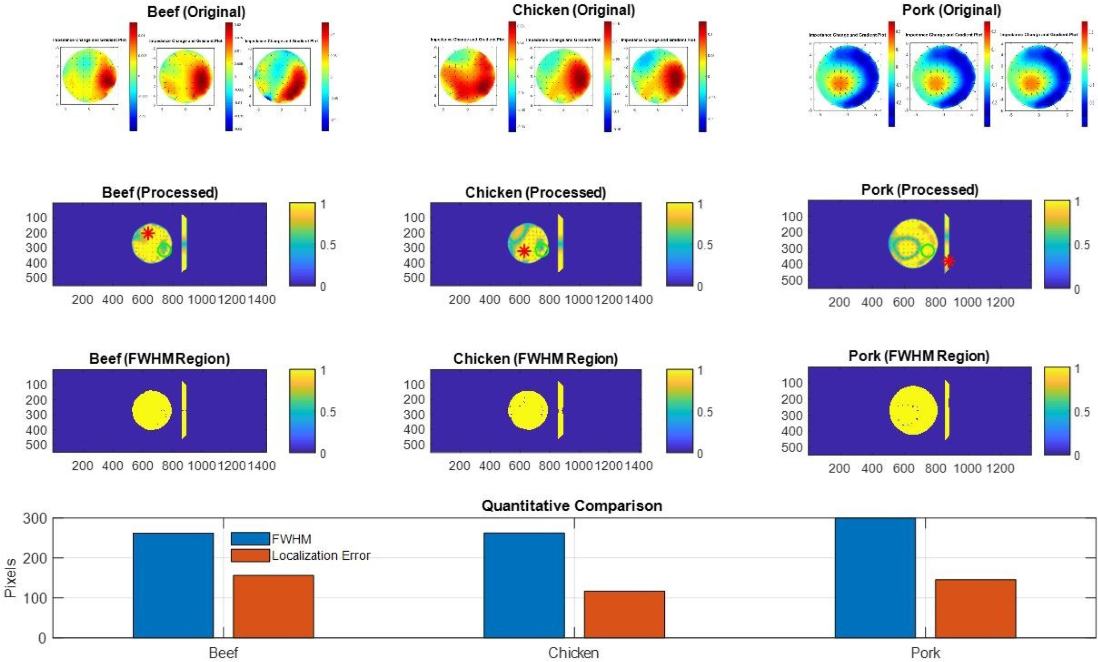
Figure 15:
Comparison of EIT reconstructions and spatial resolution metrics: FWHM and localization error.