
Table 1:
Summarised composition of fat phantom.
| Materials | Concentration (% w/w) |
|---|---|
| Demineralised water | Solvent |
| PVA | 10 |
| Beeswax | 40 |
| Activated carbon | 1 |
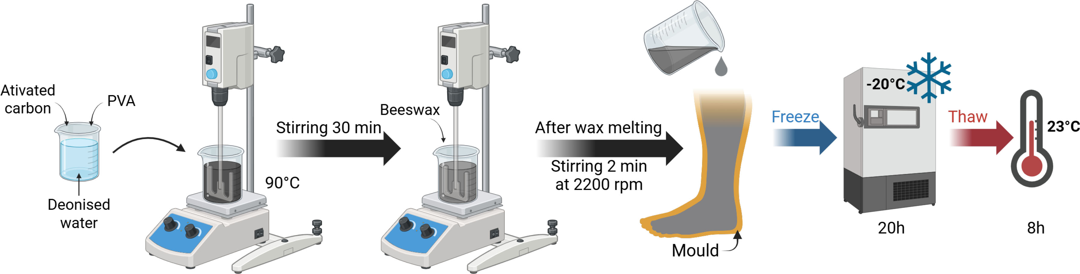
Figure 1:
Fat phantom preparation steps. Created with Biorender.
Table 2:
Summarised composition of muscle phantom.
| Materials | Concentration (% w/w) |
|---|---|
| Demineralised water | Solvent |
| PVA | 15 |
| Agar | 1.5 |
| Graphite | 10 |
| NaCl | 0.3 |
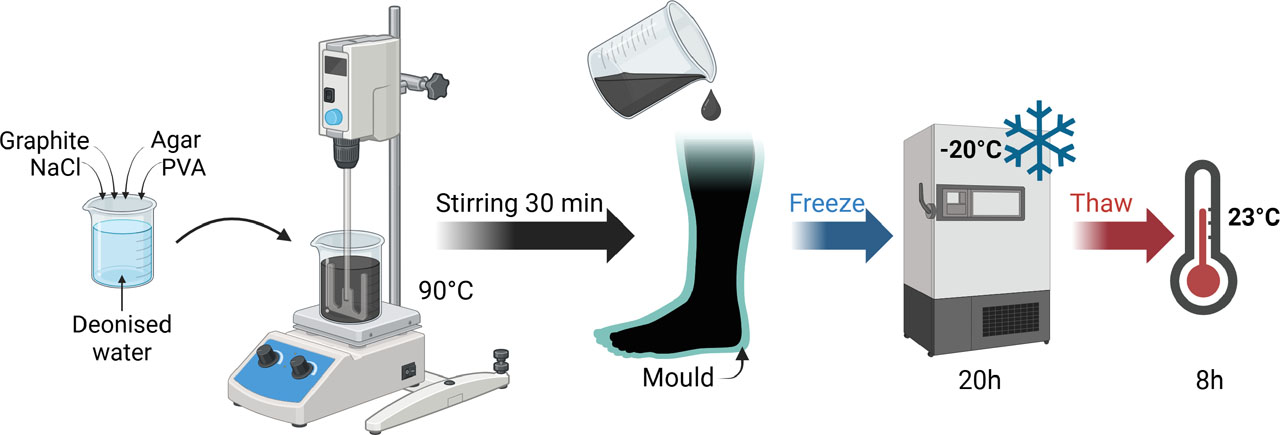
Figure 2:
Muscle phantom preparation steps. Created with Biorender.
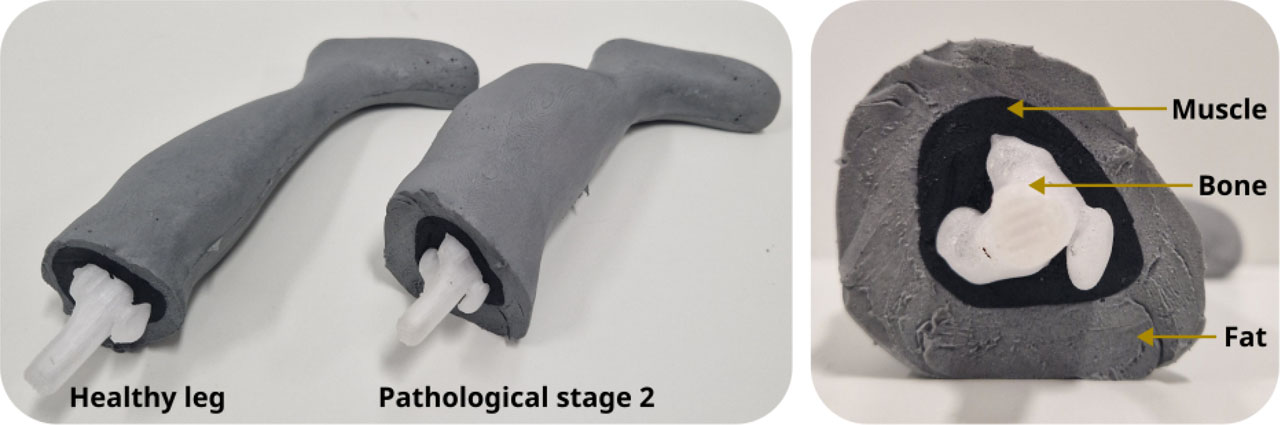
Figure 3:
Healthy and pathological leg phantoms constituted by 3 layers: bone, muscle and fat.
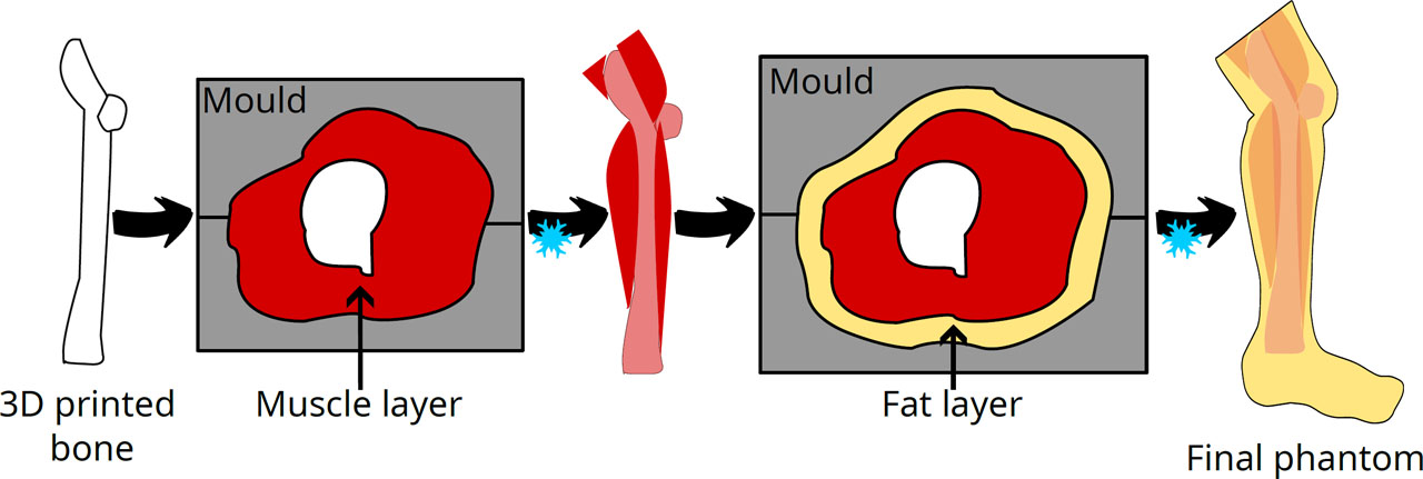
Figure 4:
Fabrication steps of the anthropomorphic phantoms.
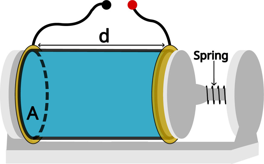
Figure 5:
Schematic of a standard measuring cell. Length d = 50 mm, inner surface area A = 4.52 cm2.
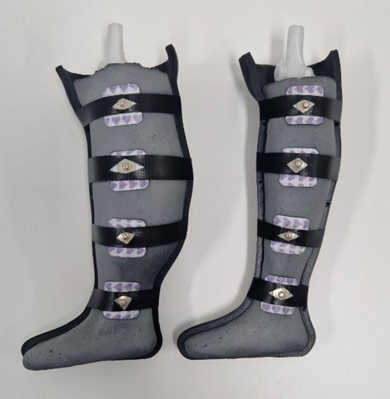
Figure 6:
Anthropomorphic leg BIS measurement setup.
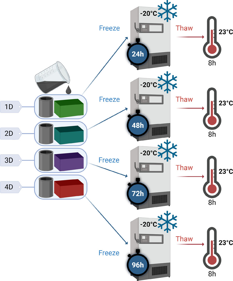
Figure 7:
Preparation of samples for the study of the effect of cycle duration on the properties of PVA-C – ‘xD’ is used as a diminutive for ‘x’ days of freezing. Created with Biorender.
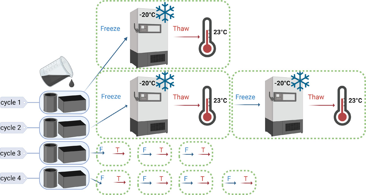
Figure 8:
Preparation of samples for the study of the effect of the number of cycles on the properties of PVA-C. Created with Biorender.
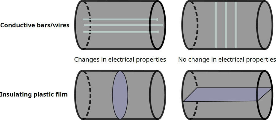
Figure 9:
Methods for reproducing anisotropy in the muscle phantom.
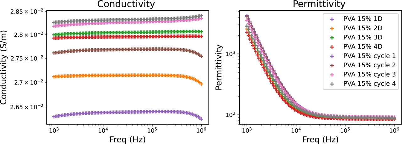
Figure 10:
Electrical properties of PVA-C as a function of the duration of the freezing cycle and the number of cycles.
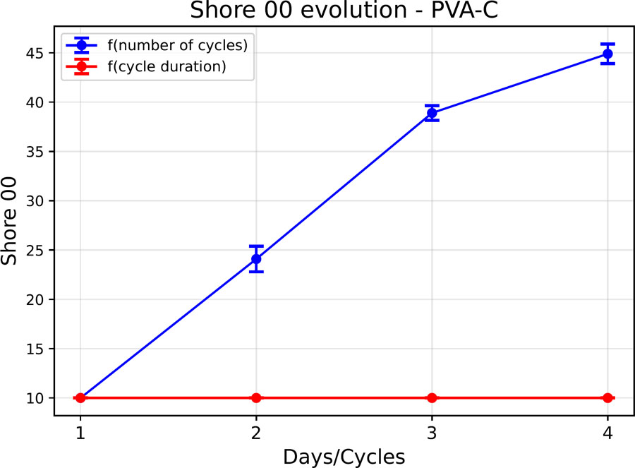
Figure 11:
Shore 00 hardness evolution of a PVA-C sample.
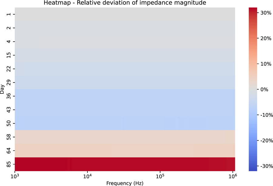
Figure 12:
Heatmap – Relative deviation of the impedance modulus as a function of frequency – case of sample storage under vacuum in a refrigerator (4 °C).
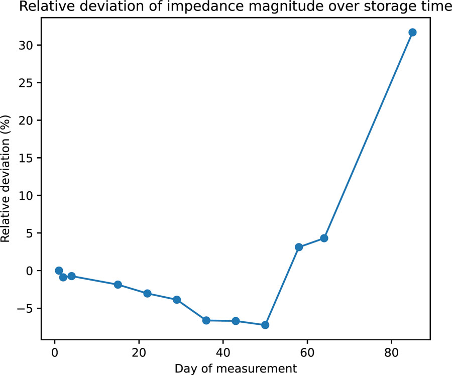
Figure 13:
Average relative deviation of the impedance modulus over time – case of sample storage under vacuum in a refrigerator.
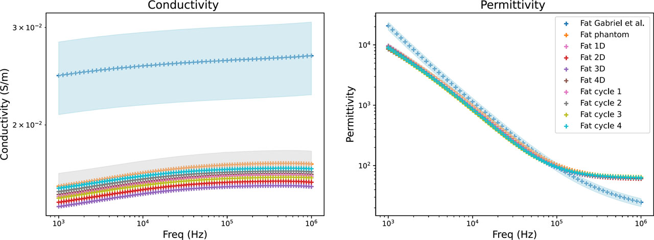
Figure 14:
Electrical properties of fat phantom: literature data (blue), mean values of the developed fat phantom (orange), and their variability range (grey). The influence of freezing duration (Fat xD) and number of freeze/thaw cycles (Fat cycle x) is also shown.
Table 3:
Relative difference between the electrical properties of the developed fat phantom (Fat 1D data) and the reference values reported by Gabriel et al. [23].
| Frequency | Conductivity | Permittivity |
|---|---|---|
| 1 kHz | –39,53% | –53,30% |
| 10 kHz | –38,72% | –22,77% |
| 100 kHz | –38,28% | 0,40% |
| 1 MHz | –39,40% | 153,73% |
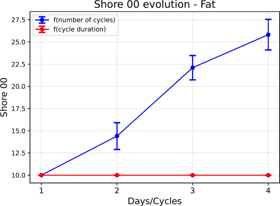
Figure 15:
Evolution of the shore 00 hardness of the fat phantom as a function of the cycle parameters.
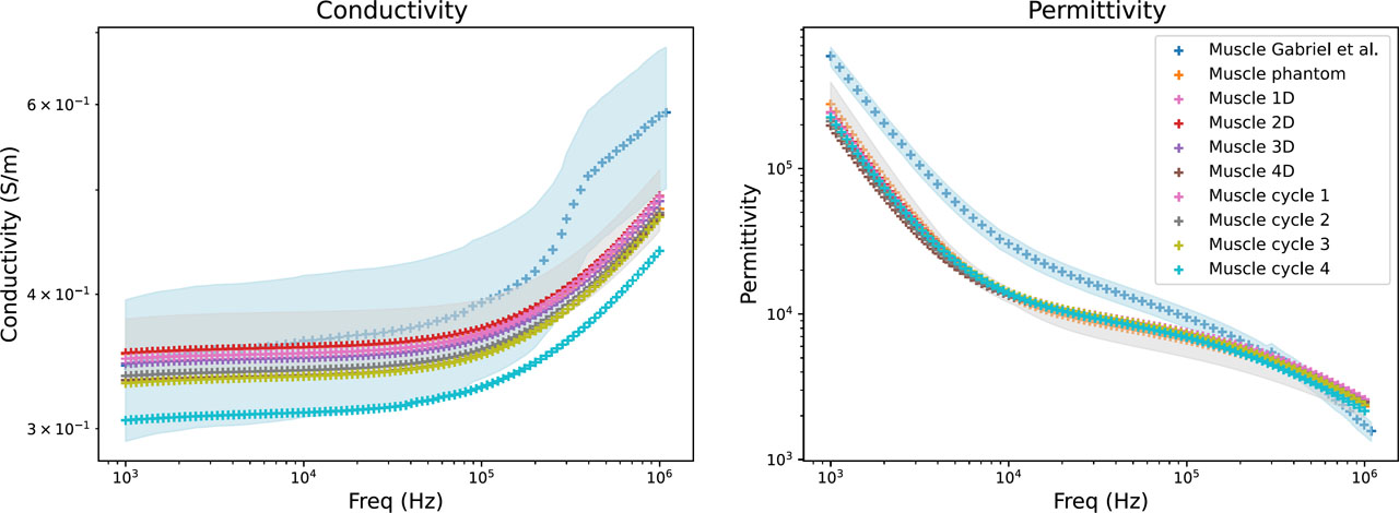
Figure 16:
Electrical properties of muscle phantom: literature data (blue), mean values of the developed muscle phantom (orange), and their variability range (grey). The influence of freezing duration (Muscle xD) and number of freeze/thaw cycles (Muscle cycle x) is also shown.
Table 4:
Relative difference between the electrical properties of the developed muscle phantom (Muscle 1D data) and the reference values reported by Gabriel et al. [23].
| Frequency | Conductivity | Permittivity |
|---|---|---|
| 1 kHz | 1,43% | −59,32% |
| 10 kHz | −2,61% | −53,58% |
| 100 kHz | −6,37% | −21,24% |
| 1 MHz | −15,88% | 50,43% |
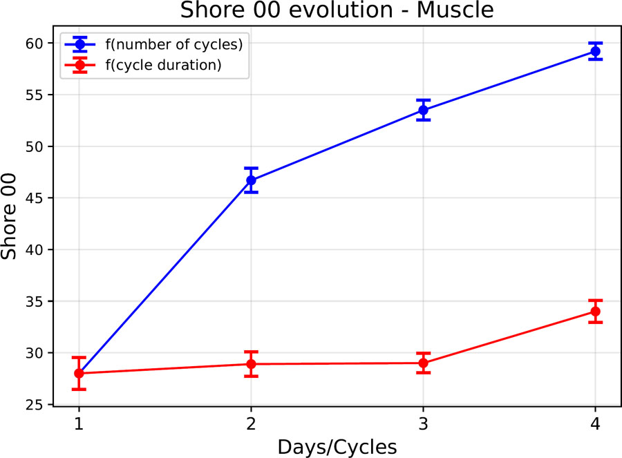
Figure 17:
Evolution of the shore 00 hardness of the muscle phantom as a function of the cycle parameters.
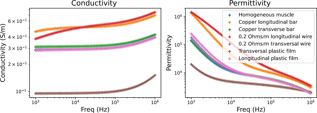
Figure 18:
Comparison of electrical properties between the homogeneous muscle model and anisotropic variants.
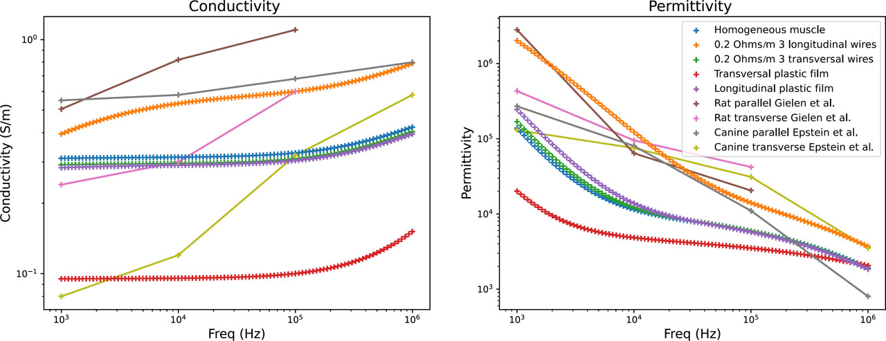
Figure 19:
Comparison of the electrical properties of the homogeneous muscle model, anisotropic variants, and data from the literature.
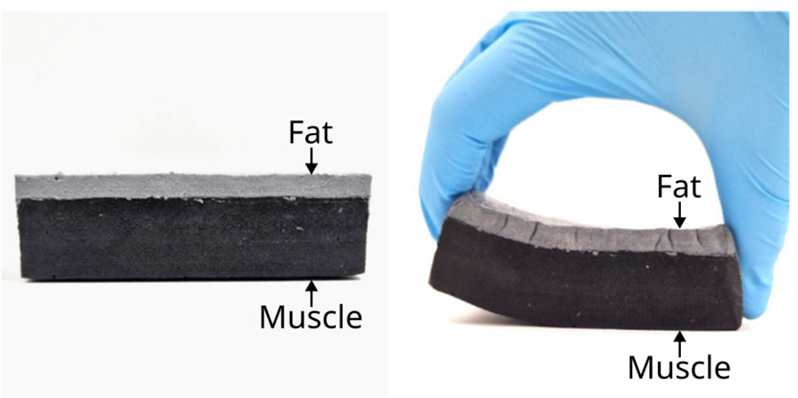
Figure 20:
Connection between the muscle layer (black matter) and the layer of fat phantom (grey matter).
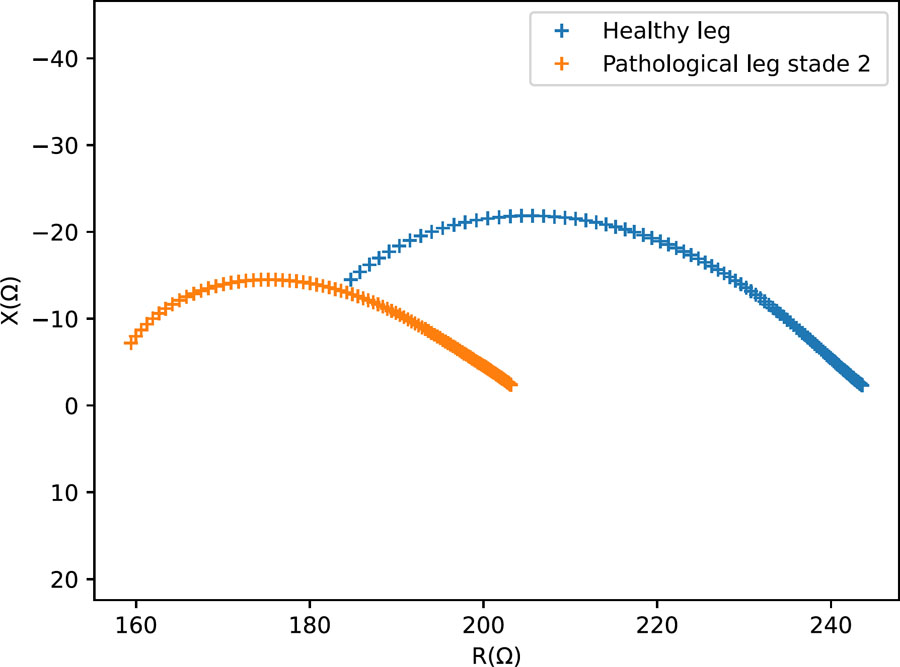
Figure 21:
Nyquist diagram – Measurements on small-scale physical models representing a healthy and lymphedema-mimicking leg configurations.