
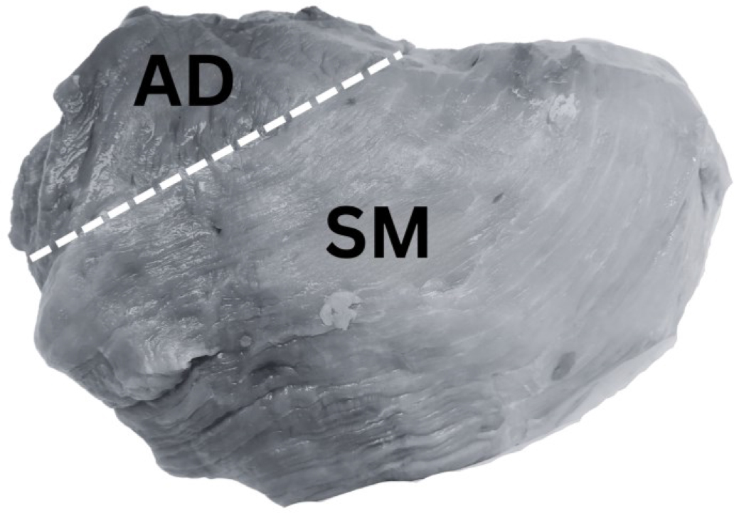
Fig. 1.
The two different muscles, for which bioimpedance, ultimate meat pH and CIELAB color values were measured. AD: adductor muscle, SM: semimembranosus muscle.
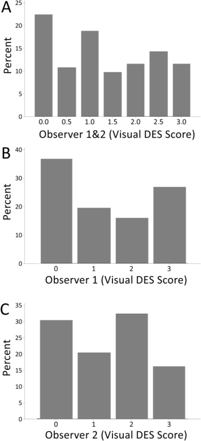
Fig. 2.
Visual DES defect scoring results of the two observers for N = 111 pork ham samples. A) the average visual scores for the two observers (note the 0.5 steps instead of integers). B, C) The distribution of the visual DES scores for the two observers separately. Both the average and individual score data sets show a sufficiently heterogeneous distribution, with all DES ranks being represented by a larger number of individuals and no heavily skewed distribution.
Table 1.
The four-rank visual DES scoring scheme for destructured ham cuts, including the semimembranosus and adductor muscle. Scoring was based on evaluating structural disintegration and visual color (adapted from [19, 24]).
| Score | 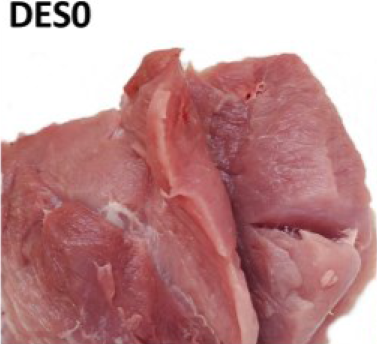 | 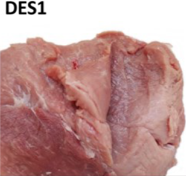 | 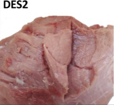 | 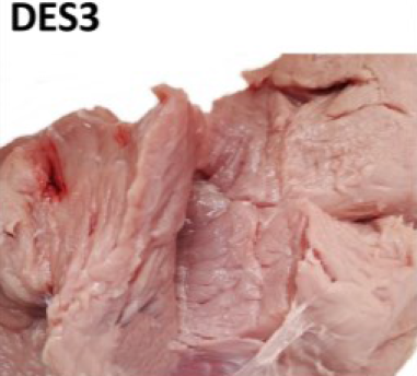 |
| Visual colour | Reddish (> 3) | From pale to reddish (1 - 3) | Very pale (1 - 2) | |
| Muscle structure defect | Compact fibre structure | Absence of fibrillar structure in the affected area Destructured meat | Absence of fibrillar structure in the affected area Soft and doughy, destructured meat Fluid exudate | |
| Area affected | None | Small areas on the surface with single patches of destructured zones | More than 50% of both muscle areas Lesions beneath the surface | |
| Observations | No visible defects | Small, pale areas on the surface | Lesion less than approx. 2cm in depth | Lesion more than approx. 2cm in depth |
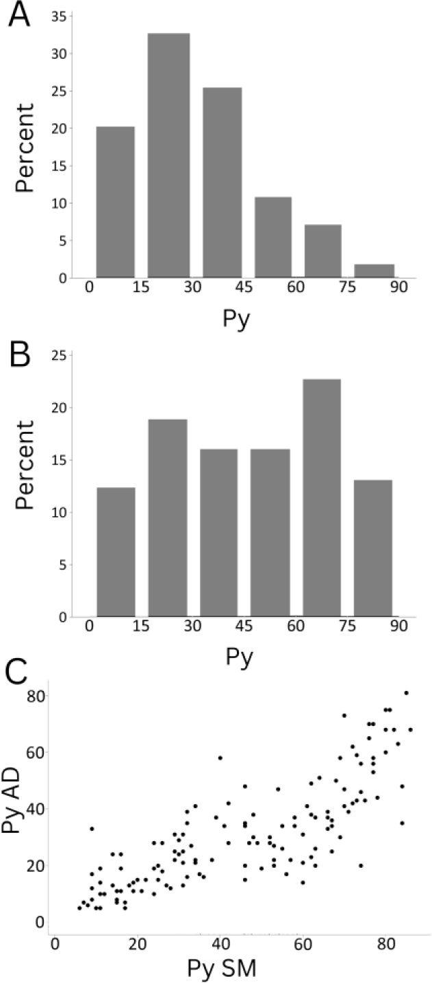
Fig. 3.
Bioimpedance response (Py parameter) distribution for two ham muscles, which were also included with the more global visual DES evaluation. A) Py parameter distribution for the AD muscle location. B) Py parameter distribution for the central SM location. C) Correlation plot of Py values scores for SM and AD testing indicating a strong correlation (r = 0.8).
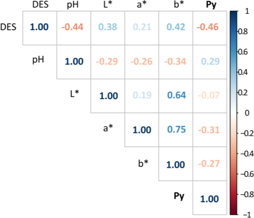
Fig. 4.
Correlation coefficients between visual destructured (DES) score and bioimpedance (BI) measurements, pHu, and CIELAB for the AD muscle. All shown correlations were found to be significant at (P < 0.05), except Py vs L* with P = 0.39.
Supplementary Table 1.
Estimated coefficients of the model statistics with P values.
| Estimate | SE | tSTAT | P - Value | |
|---|---|---|---|---|
| (Intercept) | −82.022 | 74.573 | −1.0999 | 0.274 |
| pHu | 17.343 | 13.121 | 1.3217 | 0.189 |
| L* | 2.3323 | 1.5671 | 1.4883 | 0.139 |
| a* | 0.85357 | 0.38534 | 2.2151 | 0.029 |
| b* | 0.21135 | 0.089393 | 2.3643 | 0.02 |
| Py | −0.83391 | 0.27336 | −3.0506 | 0.003 |
| pHu x L* | −0.54006 | 0.2669 | −2.0235 | 0.045 |
| pHu x Py | 0.11651 | 0.045719 | 2.5484 | 0.012 |
| L* x Py | 0.0033977 | 0.0011399 | 2.9807 | 0.003 |
| L*2 | 0.0054231 | 0.0029521 | 1.837 | 0.069 |
| a*2 | −0.035111 | 0.013828 | −2.5392 | 0.012 |