
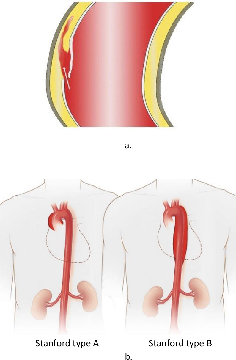
Fig. 1
a) Intimal tear in the aorta [2]. b) Aortic dissection types (Stanford system) [3].
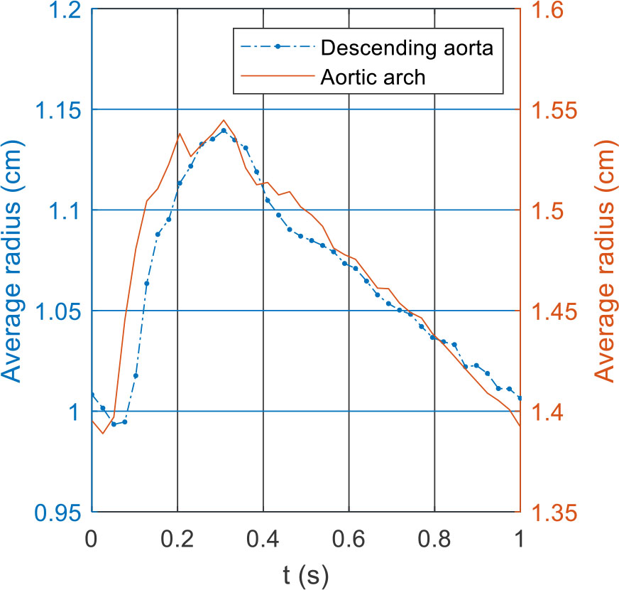
Fig. 2
The spatial average time-dependent cross-sectional radius of the aortic arch and the descending aorta during one cardiac cycle.
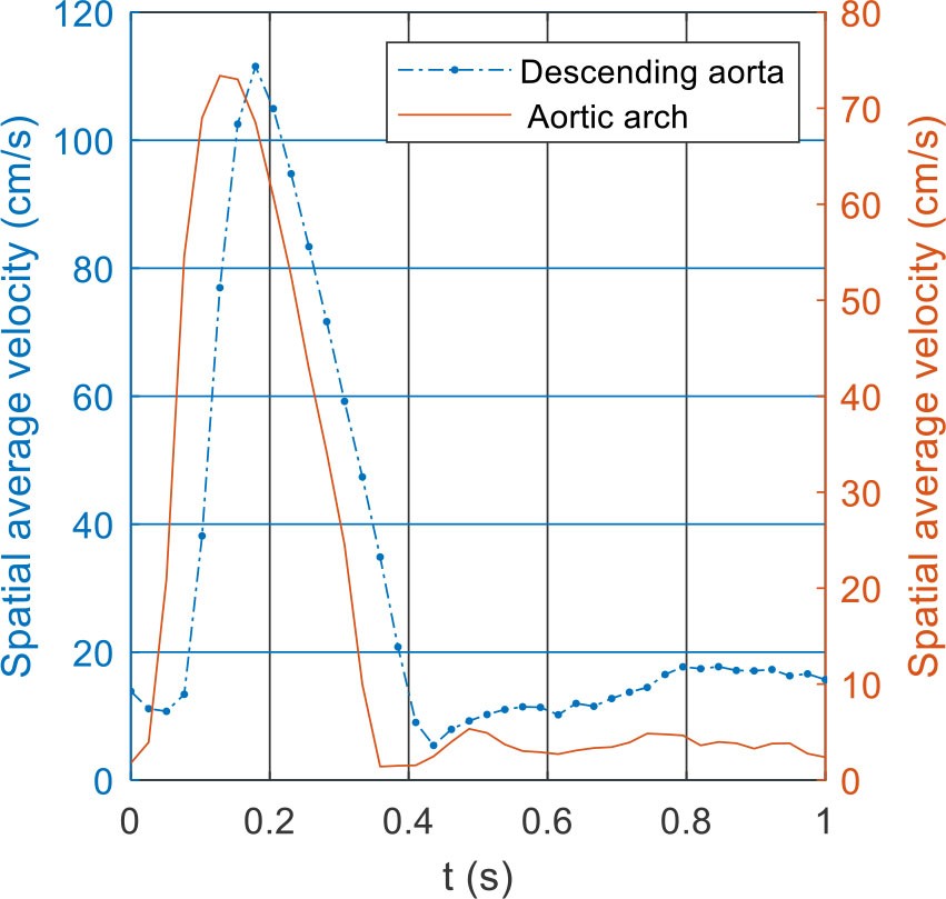
Fig. 3
The spatial average time-dependent blood velocity in the aortic arch and the descending aorta.
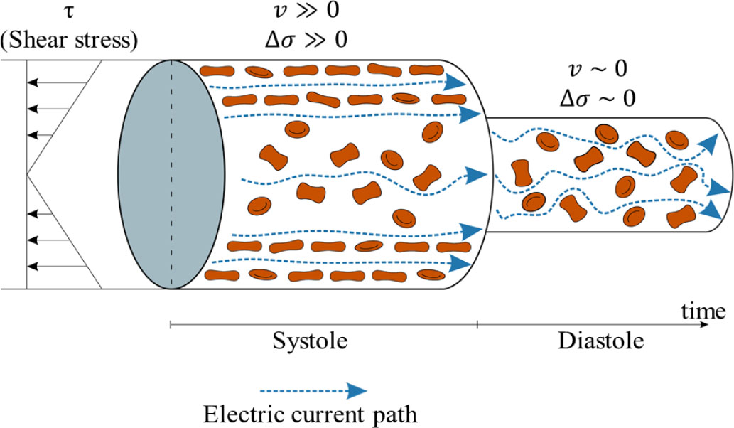
Fig. 4
Orientation and deformation of RBCs in a blood vessel during the systole and diastole.
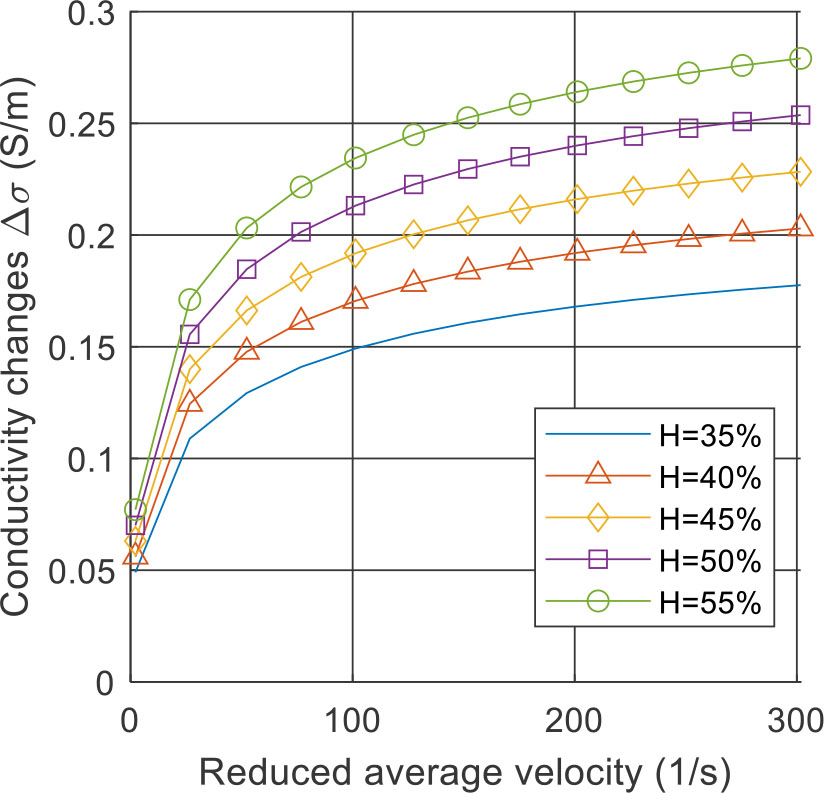
Fig. 5
The blood conductivity changes as a function of reduced average velocity 〈v/R〉 for different haematocrit (H) levels.
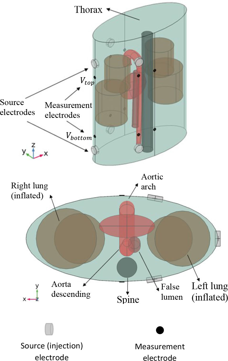
Fig. 6
Simulation model setup. a) 3D view – b) 2D bottom view.
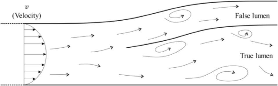
Fig. 7
Flow disturbances around the dissection in case of an aortic dissection.
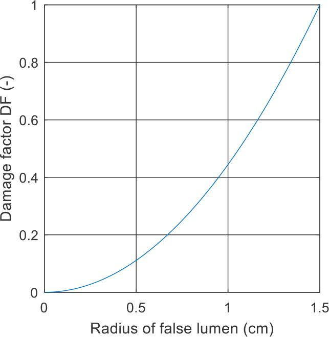
Fig. 8
Damage factor DF as a function of the radius of the false lumen.
Table. 1
Input space description for the healthy and dissected study cases.
| Cases | Variable | Distribution | Moments | Unit |
|---|---|---|---|---|
| Healthy | RTL | Uniform | [1.35 1.95] | cm |
| θH | Uniform | [1.0 1.1] | - | |
| Dissected | RTL | Uniform | [1.35 1.95] | cm |
| θH | Uniform | [1.0 1.1] | - | |
| RTL | Uniform | [0.3 1.5] | cm | |
| αFL | Uniform | [2.9 3.65] | rad |
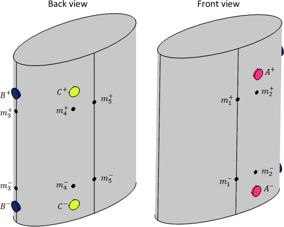
Fig. 9
Source electrode pairs and measurement electrode pairs positions.
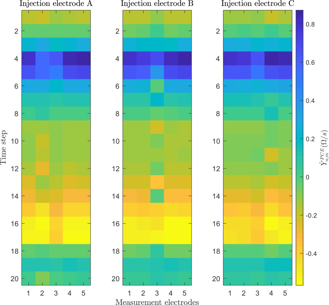
Fig. 10
Values of reflecting the discrepancy between the healthy and dissected conditions for 20-time steps and all proposed electrode combinations.
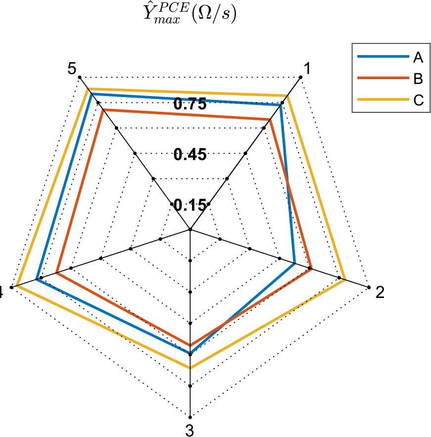
Fig. 11
Maximal discrepancy for the fourth time step and each electrode configuration. Colours show source electrodes; blue: injection from A, red: injection from B, yellow: injection from C; numbers show the measurement electrodes.
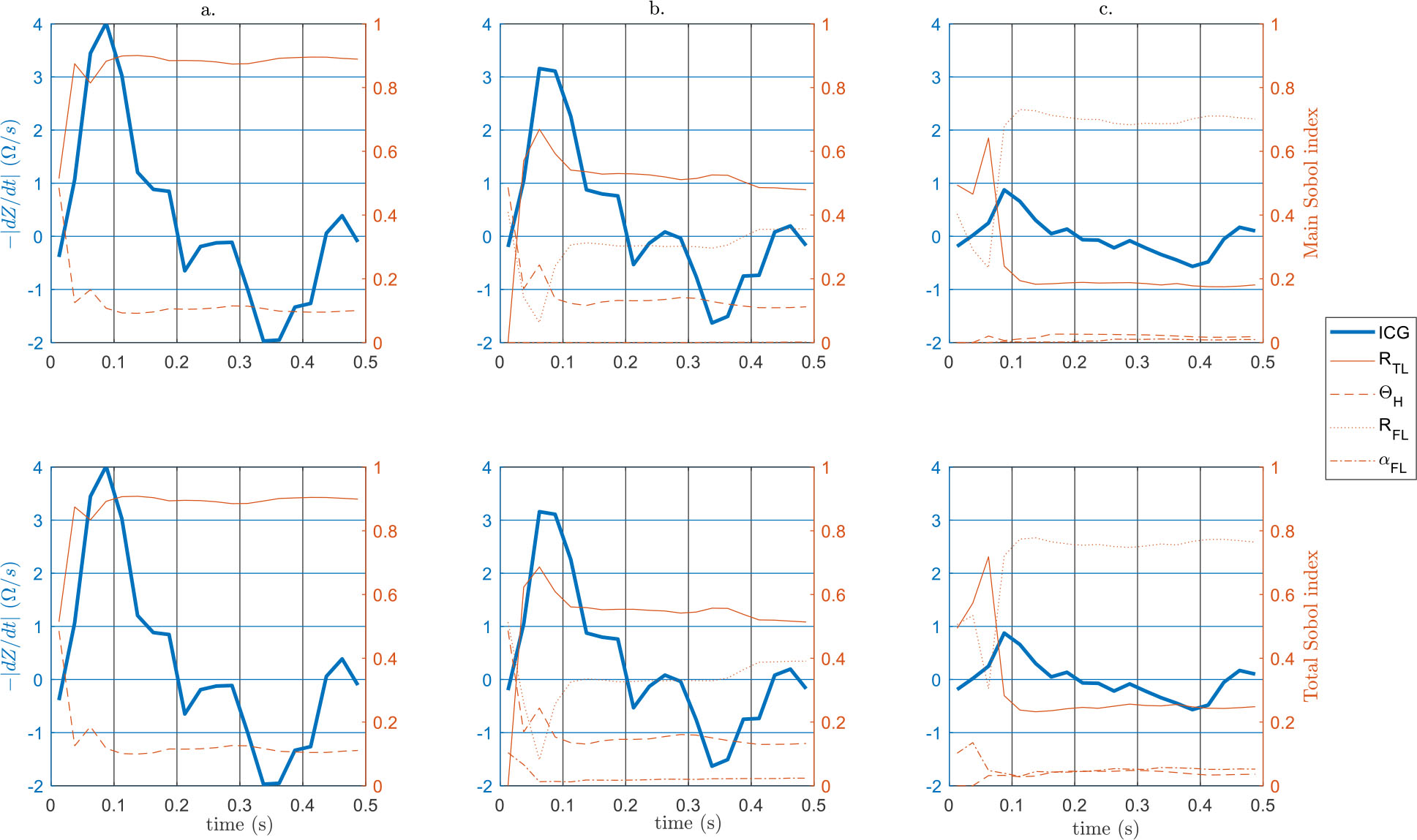
Fig. 12
Sensitivity analysis on a. , b. , c. .
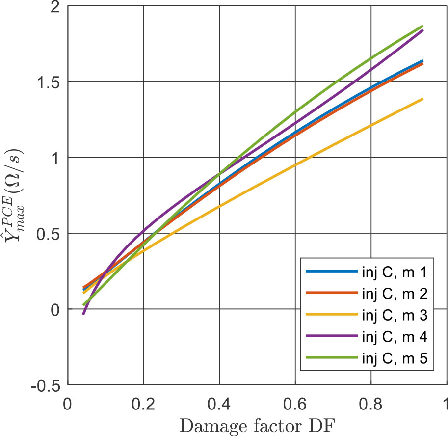
Fig. 13
Changing of by the damage factor for injection from source electrodes C (inj C) and measurement from five electrode pairs (m1 to m5).
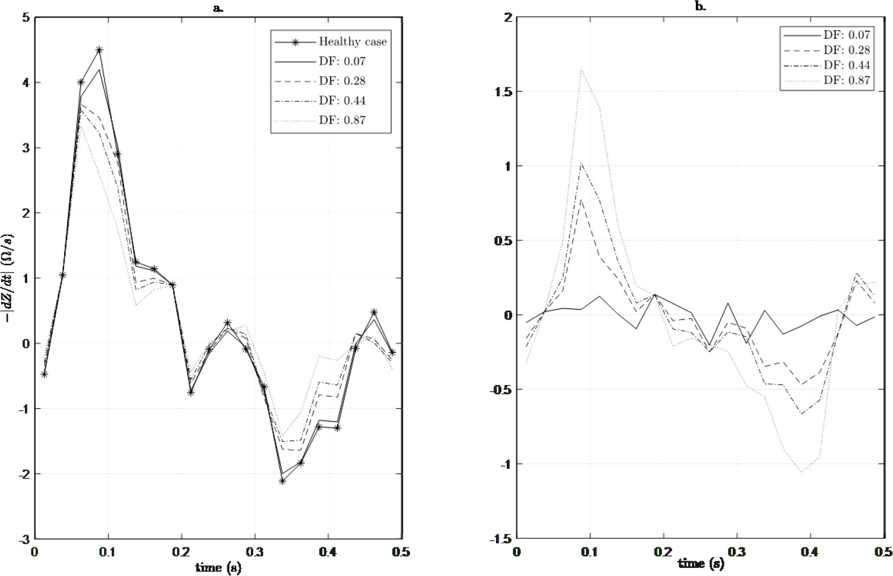
Fig. 14
a. and for different damage factors, b. for different damage factors.