
The development of a detailed, continuous mathematical model of an electrical-impedance-spectroscopy (EIS) measurement of human skin requires knowledge of both the EIS probe design as well as the properties of the adjacent skin layers. While the former is straightforward, the latter is more demanding due to the inherent complexity of human skin. This complexity arises from the form and functionality of human skin.
In essence, human skin comprises multiple layers of cells and tissues; these can be grouped into three main layers with their own thicknesses and electrical properties, as illustrated in Fig. 1: (i) a stratified, cellular epidermis; (ii) an underlying dermis made up of connective tissue that is separated from the epidermis through the dermo-epidermal junction; and (iii) the hypodermis, also known as the fatty subcutaneous layer or adipose tissue. Each of these three layers, in turn, consist of one or more sublayers; e.g., epidermis of thin skin comprises stratum corneum, stratum granulosum, stratum spinosum and stratum basale. Besides natural variations between individuals that result in differing thicknesses and electrical properties, other factors come into play such as aging, skin moisture and variation of blood flow due to ambient conditions.
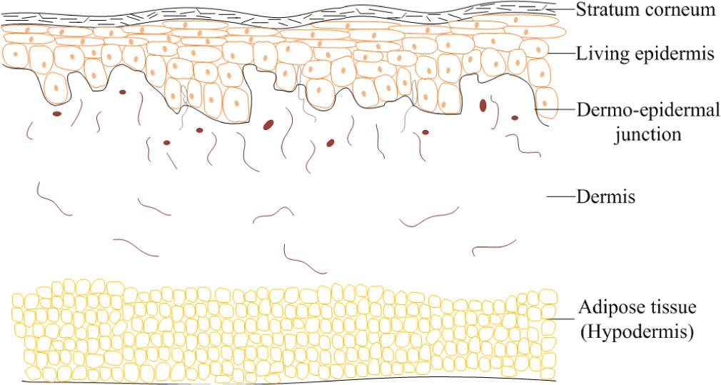
Schematic of skin layers.
In our earlier work, we derived a mathematical model based on conservation of charge for EIS measurements of human skin [1,2,3] between 1 kHz and 1 MHz by grouping the skin layers into three layers: viz., stratum corneum (SC), viable skin (VS) and adipose tissue (AT). The model, which was calibrated and validated with experimental EIS measurements, was solved numerically [1,2,3] and semianalytically [3] in the entire frequency domain and analytically [2,3] at around 1 kHz. Similar continuous models have also been solved numerically [4,5,6,7,8].
Here, we extend our previous work by generalizing the mathematical model and its solution to account for n layers and m electrodes, as shown in Fig. 2. We then demonstrate the model for three layers with a four-electrode probe, one sense with one or multiple injection electrodes, by verifying with the full set of equations solved numerically and validating with experimentally measured impedance data from an earlier study [9].
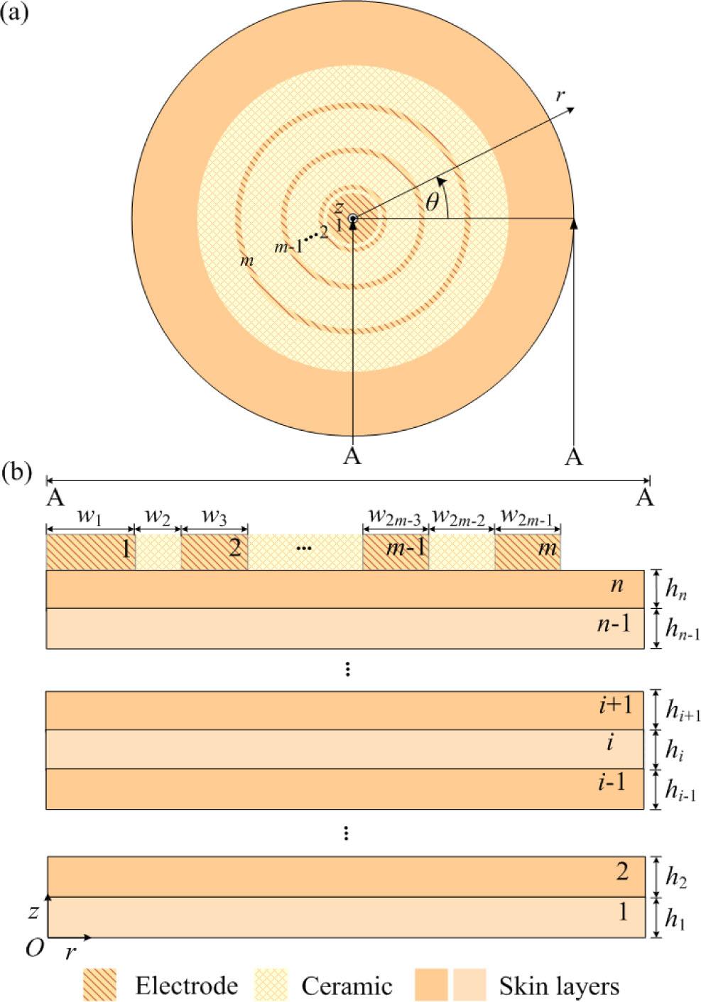
Schematic of skin comprising n layers and a circular EIS probe with m electrodes.
The potential distribution, current density and measured impedance in cylinder coordinates [3] in the skin can be written as
subject to the following external boundary conditions for j = 1, …, m electrodes:
and constitutive relations for the individual skin layers, i = 1, …, n:
The radii, Rj, for the electrodes are defined for j = 1, …, m:
For convenience, we also define the cumulative height, 𝓗i, of skin layer i = 1, …, n:
In the above equations, r and z are the cylindrical coordinates (see Fig. 2), Φ is the complex-valued potential, Jr and Jz are the current densities in the r and z direction respectively, m and n are the number of electrodes in the EIS probe and layers of skin respectively; σi,eff,
σ(i) are the effective, complex-valued electrical conductivity, the relative permittivity and conductivity of layer i, respectively; ε0 is the relative permittivity of vacuum, i is the imaginary unit, ω = 2πν is the angular frequency, ν is the frequency, Z is the impedance, Vj is the prescribed potential at a given electrode, j; wj is the width of or between an electrode as illustrated in Fig. 2 and hk is the height of skin layer k.
Note that we do not solve for the potential distribution in the electrodes, because the potential drop there is negligible [3].
Let’s start by exploiting that the current density distributions underneath the m electrodes are near-to constant because of the high resistance to current of the stratum corneum in the considered frequency range [3]. This allows us to rewrite the boundary conditions, Eqs. 5-7, between the probe and the uppermost skin layer n, stratum corneum, as (we drop the subindex `eff’ for notational convenience in the analysis)
where U() denotes the Heaviside function and Ij is the total current at the jth electrode; the area of the jth electrode is
Strictly speaking, we are no longer solving exactly the same set of equations with the rewritten boundary condition, Eq. 15, whence we will refer to our generalized solution as approximate in nature.
From the conservation of current for the entire system, we know that
We can now proceed with a Hankel transform of zeroth order, H0 {}, for the potential,
which is ideally suited for the axisymmetric Laplace equation, Eq. 1, on our unbounded domain:
with the solution for each skin layer, i,
and its z-derivative,
here, Ai (ξ) and Bi (ξ) are two functions that we will soon determine, Δ is the Laplace operator, and J0 is the 0th - order Bessel function of the first kind. Between layers, we know that the flux and potential are continuous; i.e.
for 1 ≤ i ≤ n − 1. In addition, we need to satisfy the two boundary conditions at z = 0,
and at z =𝓗n,
with
here we have used that the Hankel transform of zeroth order of a Heaviside function is defined as
with J1 and a (> 0) denoting the 1st-order Bessel function of the first kind and a constant respectively [10].
Note that we have also switched to the subscript, k, in the summation over the electrodes in Eq. 25 to avoid confusion with the matrix notation we will introduce later. Let us solve the potential of the first layer and then work our way up to the uppermost n-th layer. Starting with the boundary condition, Eq. 24 at z = 0, we have
which results in
with
the role of e2ξ𝓗0 Λ1 (=1) will become apparent as we proceed with our analysis. Proceeding to the other boundary condition for the first layer, Eq. 23, we have for z = 𝓗1 that
i.e.,
from which we find (N.B.: 𝓗1 = h1)
Moving on to the second layer, we find after satisfying the continuity of flux at z = 𝓗1,
that
with
Between the second and third layer, z = 𝓗2, we require continuity of the potential,
which reveals
Let us explicitly continue with the third layer and then generalize the solution for layer i, where 1 ≤ i ≤ n − 1. In the third layer, we find
and
with
after satisfying the boundary conditions with the second and fourth skin layer.
We can now generalize the solution as
and
for 1 ≤ i ≤ n − 1, with
for i = 1, and the recursive formula for Λi,
for 2 ≤ i ≤ n − 1.
In the n-th layer, we find after satisfying the continuity of potential with the n − 1 layer and the boundary condition, Eq. 25, between the electrodes and the uppermost skin layer,
by setting
and
from the uppermost boundary condition at z = 𝓗n for layer n:
At this stage, we can write the local, pointwise transformed potential in layer i as
In this expression, the coordinate, z, is bounded for each layer as
Now, taking the inverse Hankel transform,
we find the local potential distribution throughout the viable skin as
and
We have m + 1 unknows: I1 to Im and c; the latter constant provides a reference point for the potential since we have in the approximate solution only solved for Neuman boundary conditions. In order to determine the unknowns, we return to our pointwise Dirichlet boundary conditions for the potentials underneath the electrodes, Eq. 5, and rewrite Eqs. 54 and 55 in terms of the average potential underneath the jth electrode in the uppermost skin layer, n:
or, after integration once, as
where
During the integration, we used that
The overall conservation of current, Eq. 17, allows us to reduce the number of unknowns by one, as we can write
Introducing the expression for the current of the outermost electrode, Im, into Eq. 57, yields the following system of m linear equations:
with
and
Once the linear system of equations together with the improper integrals given by Eq. 66 have been solved, the impedance can be found from
assuming that V0 is set as reference potential for the measurements and that the first electrode is used as the sense. We’ll give one example of this in the next subsection. If the electrode system is different, one needs to couple the right current with the given potential to determine the impedance.
This solution corresponds to EIS measurements in our earlier experimental study [9] and the model thereof with skin encompassing three layers (n=3): stratum corneum, viable skin and adipose tissue, as illustrated in Fig. 3.
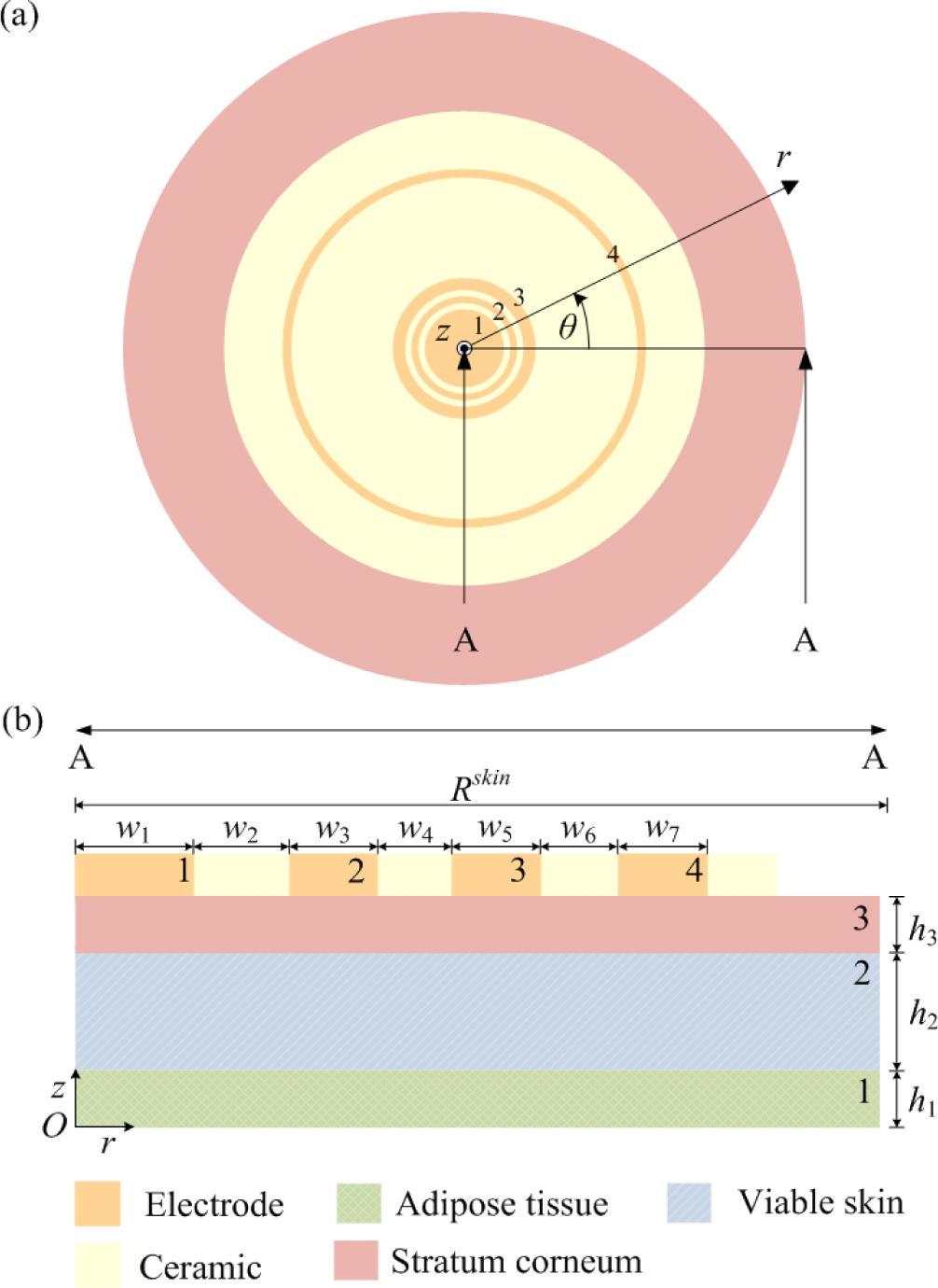
Schematic of a 4-electrode probe and skin modeled as a three-layer entity.
Here, the first electrode is the sense, the second serves as the guard, the third is the second inject with a potential set as αV0 and the fourth is the primary inject with a potential of V0; α is referred to as a depth setting on the probe; i.e. m=4. The boundary conditions for the complexvalued Laplace equation reduce to
and
Our generalized solution becomes
where
The individual average currents for the four electrodes are as follows (we have dropped the comma notation for the subscripts of the elements in A for notational convenience; b = [0, 0, αV0, V0]T):
and
with the constants
and
Note that the entries, Aij, in the above expressions entail solving the improper integral, Eq. 66, twelve times.
The parameters are given in Table 1.
Base-case dimensions and material parameters for the 4-electrode probe and 3 skin layers (n=3, m=4). (The outer radius of the skin is only used in the numerical solution for verification purposes.)
| Current detection width, w1 | 1 mm | [2] |
| Ceramic width, w2, w4, w6 | 0.15, 0.15, 1.9 mm | [2] |
| Guard width, w3 | 0.3 mm | [2] |
| Secondary inject width, w5 | 0.5 mm | [2] |
| Primary inject width, w7 | 0.5 mm | [2] |
| Outer radius of the probe, R | 4.5 mm | [2] |
| Outer radius of the skin, Rskin | 20 mm | |
| Stratum corneum thickness, h3 | 14 μm | [11] |
| Viable skin thickness, h2 | 1.2 mm | [11] |
| Adipose tissue thickness, h1 | 1.2 mm | [11] |
| Inject voltage, V0 | 0.05 V | [2] |
| Depth setting, α | 0.1 | [2] |
| Electrical permittivity in vacuum, ε0 | 8.85 ×10⁷ Fm-1 | [12] |
For the skin, we can write the constitutive relations for the relative permittivity and the conductivity (S m-1) as follows [9] based on the dimensionless logarithmic frequency, N = log10(ν/1 Hz).
In the stratum corneum, i=3, we have
In the viable skin, i=2, we have
And finally in the adipose tissue, i=1, we have
We solve the model, Eqs. 1-13, in the finite-element solver Comsol Multiphysics 5.2a [13] and the approximate semianalytical model, Eqs. 79-88, and its pointwise solution in the skin layers, Eq. 55, in the general-purpose numerical software Matlab R2015 [14].
We have thus far derived an approximate semianalytical solution of the mechanistic model for EIS measurements of human skin. Let us proceed by validating it with a previous study comprising 120 young subjects (24 ± 3 years old), who had no known skin diseases or allergies; and were asked to abstain from applying moisturizers on the day of the measurements. Before the measurements were taken on the volar forearm of the subjects, their skin was soaked in physiological saline solution (at a concentration of 0.9% sodium chloride in mass) for 1 min [9].
From the full set of 35 impedance measurements distributed logarithmically from 1 kHz to 2.5 MHz, we select a subset within the frequency range of 1 kHz to 1 MHz and a depth setting, α, of 0.1 for this validation. Overall, as can be inferred from Fig. 4, we see a good agreement between the semi-analytical solution (lines) and the measured means (symbols) for both the magnitude and the phase throughout the frequency spectrum. Furthermore, the semi-analytical solutions for ± 1 standard deviation for the thickness of stratum corneum (dashed lines) follow the ± 1 standard deviations from the experiments (error bars) well for the magnitude and manages to capture the increasing variations, larger standard deviations, in the measured phase as we move towards 1 MHz.
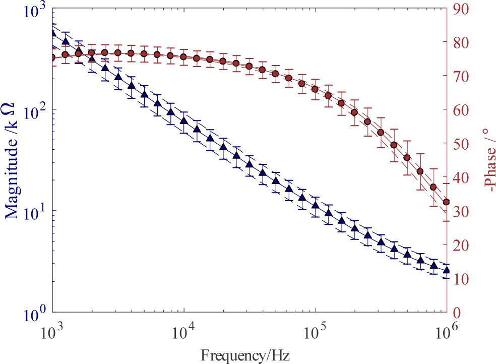
The mean magnitude (▲) and phase (•) from the experimental EIS measurements [9] with the error bars indicating one standard deviation. The lines are the predicted counterparts from the approximate semi-analytical solution, where (–) represent a thickness of 14 μm SC and (- -) denotes a thickness of either 11 or 17 μm. These values for the thickness of SC correspond to the mean and ± one standard deviation.
As we proceed to verify the individual currents at each electrode, we observe that the real part has good agreement throughout the frequency range, while the imaginary part has while the imaginary part has good agreement for most of the range and has a slight deviation of around 9% towards 1 MHz, as depicted in Fig. 5. By employing Hankel transform, we obtain a lower error with our analytical solution, as compared to the previously used analytical solution [2].
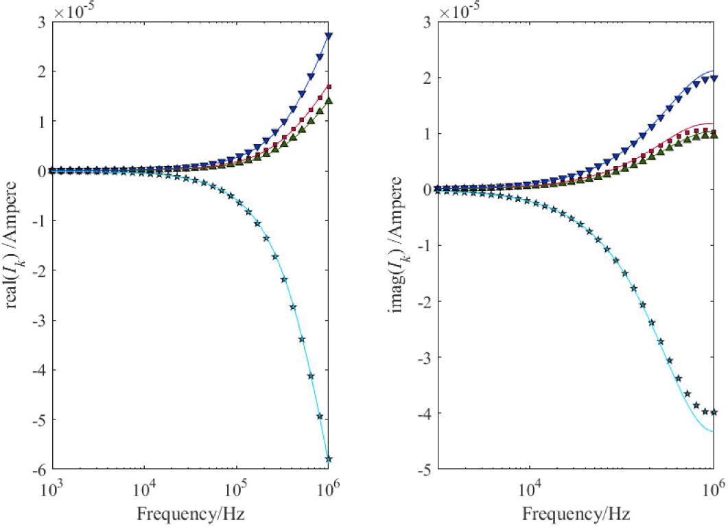
The individual currents, Ik, in terms of their (a) real and (b) imaginary parts for the numerical solution of the complete model (symbols) and the corresponding analytical counterpart (lines), for I4 (★), I2 (▲), I1 (■) and I3 (▼).
One advantage of the analysis is that we can estimate not only the overall measured impedance in the form of the magnitude and phase, but also quantify the local potential distribution throughout the various skin layers of interest. It turns out that the approximation of the uppermost boundary conditions between the stratum corneum and the electrodes is valid throughout the frequency spectrum we consider here, as illustrated in Fig. 6 at 1 MHz. In particular, we are able to capture the one-dimensional current in the stratum corneum in the z-direction, which has also been shown through a scaling analysis [3].
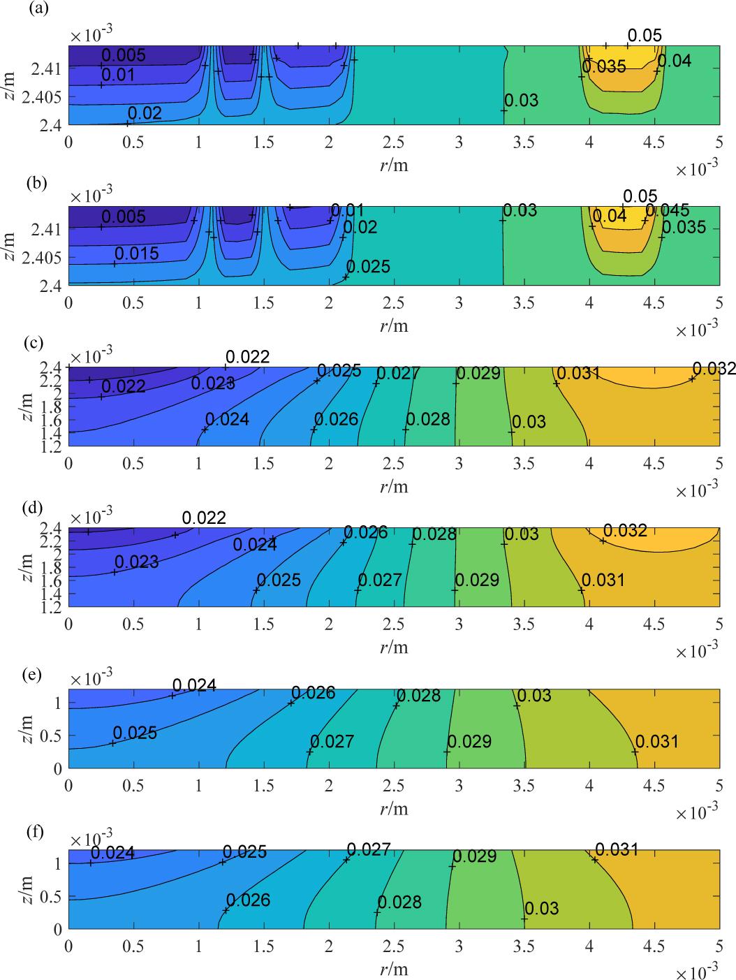
The absolute value of the potential distribution at 1 MHz for n=3 and m=4: The numerical solution of the full set of equations for SC (a), VS (c), and AT (e); and approximate semianalytical solution for SC (b), VS (d) and AT (f).
We have secured approximate semi-analytical solutions of a generalized continuous mathematical model that considers EIS with a probe comprising m electrodes and the adjacent skin divided into n layers.
Good agreement for the frequency range of 1 kHz to 1 MHz was found between the semi-analytical solution and the numerical solution of the full set of equations assuming a three-layer skin entity as well as an experimental series of 120 subjects that were measured with an EIS probe.
This particular probe has four electrodes – one sense, one guard and two injects – but we note that one can easily modify the boundary conditions such that one can model different types of measurements, such as a pure two-point measurement.
These solutions lend themselves well to studies that seek to calibrate the material properties of more skin layers than the three we consider here. In particular, it would be of interest to split up our viable skin into living epidermis and dermis since they should have significantly different material properties.
Finally, with regards the semi-analytical nature of the solutions, we note that if we manage to find closed-form expressions – even approximate ones – of the improper integrals, Aij, that arose when we pulled the solution back to the original cylindrical domain, we would be able to achieve an analytical solution that does not require any numerical integration at all.