
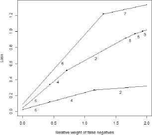
Figure 1.
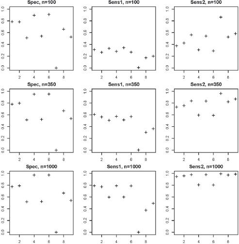
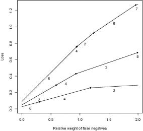
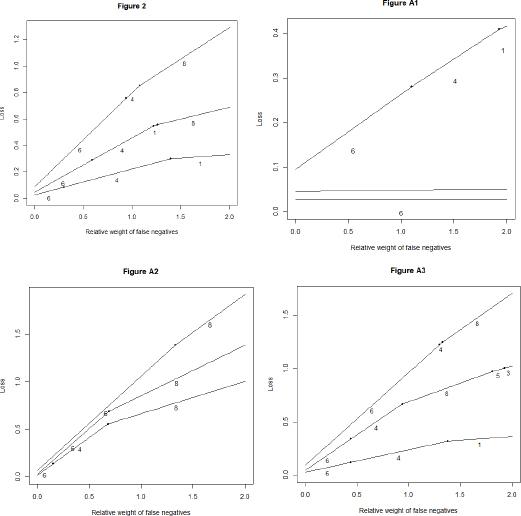
Figure 2.
Results of the main model comparison_
| Method 1 | Method 2 | Method 3 | Method 4 | Method 5 | Method 6 | Method 7 | Method 8 | Method 9 | ||
|---|---|---|---|---|---|---|---|---|---|---|
| n=100 | Spec | .79 [.004] | .78 [.004] | .51 [.005] | .89 [.003] | .54 [.005] | .91 [.003] | .00 [.000] | .66 [.005] | .53 [.005] |
| Sens1 | .31 [.005] | .27 [.004] | .33 [.005] | .28 [.004] | .34 [.005] | .27 [.004] | .01 [.001] | .17 [.004] | .20 [.004] | |
| Sens2 | .38 [.005] | .42 [.005] | .56 [.005] | .31 [.005] | .54 [.005] | .29 [.005] | .86 [.003] | .53 [.005] | .58 [.005] | |
| n=350 | Spec | .78 [.004] | .80 [.004] | .51 [.005] | .95 [.002] | .52 [.005] | .95 [.002] | .00 [.000] | .67 [.005] | .54 [.005] |
| Sens1 | .61 [.005] | .56 [.005] | .51 [.005] | .57 [.005] | .51 [.005] | .57 [.005] | .00 [.000] | .30 [.005] | .36 [.005] | |
| Sens2 | .73 [.004] | .76 [.004] | .84 [.004] | .59 [.005] | .83 [.004] | .59 [.005] | .96 [.002] | .82 [.004] | .87 [.003] | |
| n=1000 | Spec | .78 [.004] | .79 [.004] | .52 [.005] | .97 [.002] | .52 [.005] | .97 [.002] | .00 [.000] | .67 [.005] | .54 [.005] |
| Sens1 | .79 [.004] | .77 [.004] | .60 [.005] | .79 [.004] | .60 [.005] | .79 [.004] | .00 [.000] | .37 [.005] | .49 [.005] | |
| Sens2 | .95 [.002] | .96 [.002] | .98 [.001] | .80 [.004] | .98 [.001] | .80 [.004] | .99 [.001] | .97 [.002] | .99 [.001] |
Model comparison with a misspecified logistic model_
| Method 1 | Method 2 | Method 3 | Method 4 | Method 5 | Method 6 | Method 7 | Method 8 | Method 9 | ||
|---|---|---|---|---|---|---|---|---|---|---|
| n=100 | Spec | .79 [.004] | .78 [.004] | .50 [.005] | .89 [.003] | .54 [.005] | .91 [.003] | 0.0 [.000] | .66 [.005] | .53 [.005] |
| Sens1 | .14 [.003] | .13 [.003] | .22 [.004] | .13 [.003] | .22 [.004] | .12 [.003] | 0.0 [.000] | .09 [.003] | .08 [.003] | |
| Sens2 | .17 [.004] | .23 [.004] | .37 [.005] | .14 [.003] | .36 [.005] | .13 [.003] | .83 [.004] | .32 [.005] | .32 [.005] | |
| n=350 | Spec | .78 [.004] | .79 [.004] | .51 [.005] | .95 [.002] | .52 [.005] | .95 [.002] | 0.0 [.000] | .66 [.005] | .53 [.005] |
| Sens1 | .43 [.005] | .38 [.005] | .45 [.005] | .33 [.005] | .45 [.005] | .32 [.005] | 0.0 [.000] | .22 [.004] | .20 [.004] | |
| Sens2 | .52 [.005] | .57 [.005] | .73 [.004] | .34 [.005] | .73 [.004] | .34 [.005] | .91 [.003] | .65 [.005] | .66 [.005] | |
| n=1000 | Spec | .78 [.004] | .80 [.004] | .52 [.005] | .97 [.002] | .52 [.005] | .97 [.002] | 0.0 [.000] | .66 [.005] | .54 [.005] |
| Sens1 | .76 [.004] | .73 [.004] | .59 [.005] | .77 [.004] | .60 [.005] | .77 [.004] | 0.0 [.000] | .36 [.005] | .35 [.005] | |
| Sens2 | .93 [.003] | .94 [.002] | .98 [.002] | .79 [.004] | .98 [.002] | .79 [.004] | .98 [.001] | .95 [.002] | .96 [.002] |
Model comparison with two effects_
| Method 1 | Method 2 | Method 3 | Method 4 | Method 5 | Method 6 | Method 7 | Method 8 | Method 9 | ||
|---|---|---|---|---|---|---|---|---|---|---|
| n=100 | Spec | .83 [.004] | .81 [.004] | .57 [.005] | .92 [.003] | .60 [.005] | .93 [.003] | 0.0 [.000] | .67 [.005] | .72 [.004] |
| Sens1 | .01 [.001] | .04 [.002] | .07 [.002] | .01 [.001] | .06 [.002] | .01 [.001] | .03 [.002] | .03 [.002] | .02 [.001] | |
| Sens2 | .02 [.002] | .08 [.003] | .11 [.003] | .01 [.001] | .10 [.003] | .01 [.001] | .37 [.005] | .21 [.004] | .02 [.001] | |
| n=350 | Spec | .83 [.004] | .82 [.004] | .58 [.005] | .97 [.002] | .58 [.005] | .97 [.002] | 0.0 [.000] | .68 [.005] | .71 [.005] |
| Sens1 | .03 [.002] | .17 [.004] | .20 [.004] | .05 [.002] | .20 [.004] | .04 [.002] | .01 [.001] | .09 [.003] | .02 [.001] | |
| Sens2 | .11 [.003] | .25 [.004] | .31 [.005] | .05 [.002] | .30 [.005] | .04 [.002] | .43 [.005] | .47 [.005] | .02 [.001] | |
| n=1000 | Spec | .82 [.004] | .82 [.004] | .57 [.005] | .98 [.001] | .58 [.005] | .98 [.001] | 0.0 [.000] | .67 [.005] | .70 [.005] |
| Sens1 | .11 [.003] | .35 [.005] | .35 [.005] | .20 [.004] | .35 [.005] | .20 [.004] | 0.0 [.001] | .13 [.003] | .03 [.002] | |
| Sens2 | .43 [.005] | .45 [.005] | .52 [.005] | .21 [.004] | .52 [.005] | .21 [.004] | .49 [.005] | .66 [.005] | .03 [.002] |
Model comparison with a stronger effect_
| Method 1 | Method 2 | Method 3 | Method 4 | Method 5 | Method 6 | Method 7 | Method 8 | Method 9 | ||
|---|---|---|---|---|---|---|---|---|---|---|
| n=100 | Spec | .78 [.004] | .78 [.004] | .51 [.005] | .89 [.003] | .54 [.005] | .90 [.003] | .00 [.000] | .66 [.005] | .53 [.005] |
| Sens1 | .76 [.004] | .72 [.004] | .57 [.005] | .77 [.004] | .60 [.005] | .78 [.004] | .00 [.001] | .37 [.005] | .47 [.005] | |
| Sens2 | .90 [.003] | .92 [.003] | .96 [.002] | .84 [.004] | .95 [.002] | .83 [.004] | .96 [.002] | .95 [.002] | .97 [.002] | |
| n=350 | Spec | .79 [.004] | .80 [.004] | .51 [.005] | .95 [.002] | .52 [.005] | .95 [.002] | .00 [.000] | .67 [.005] | .55 [.005] |
| Sens1 | .84 [.004] | .43 [.005] | .60 [.005] | .96 [.002] | .62 [.005] | .96 [.002] | .00 [.000] | .39 [.005] | .56 [.005] | |
| Sens2 | 1.0 [.000] | 1.0 [.000] | 1.0 [.000] | 1.0 [.001] | 1.0 [.000] | 1.0 [.001] | 1.0 [.000] | 1.0 [.000] | 1.0 [.000] | |
| n=1000 | Spec | .78 [.004] | .80 [.004] | .51 [.005] | .97 [.002] | .52 [.005] | .97 [.002] | 0.0 [.000] | .66 [.005] | .54 [.005] |
| Sens1 | .84 [.004] | .09 [.003] | .61 [.005] | .98 [.001] | .61 [.005] | .98 [.001] | 0.0 [.000] | .39 [.005] | .61 [.005] | |
| Sens2 | 1.0 [.000] | 1.0 [.000] | 1.0 [.000] | 1.0 [.000] | 1.0 [.000] | 1.0 [.000] | 1.0 [.000] | 1.0 [.000] | 1.0 [.000] |