
1. Introduction
The introduction or expansion of a social insurance program is one of the most essential and controversial public policy issues in both developed and developing countries. Public health insurance is a central topic of study and debate. The 2008 Medicaid expansion in Oregon and the Affordable Care Act in the United States, for instance, are leading examples of policy changes that have led to numerous academic studies and public discussions (Obama, 2016; Sommers et al., 2017).
While public long-term care (LTC) insurance is much less studied than public health insurance, public LTC systems and publicly financed formal care are important for both those who need care for themselves and for their family members, particularly female informal care-givers (in this paper LTC indicates personal care for those who need assistance for their daily activities, formal caregivers mean publicly funded caregivers, and informal caregivers are all the other types of caregivers such as family and relatives).
The effects of informal caregiving on the female labor supply have been intensively studied in health and labor economics. Lilly et al. (2007) and Bauer and Sousa-Poza (2015) reviewed studies on the impact of informal caregiving on caregivers’ labor supply and related outcomes. The estimated effects of informal caregiving on the (female) labor supply in these studies are different and heterogeneous, but both Lilly et al. (2007) and Bauer and Sousa-Poza (2015) conclude that in general, the estimated negative impacts tend to be small or modest. Another important topic in the empirical literature on LTC in economics is the relationship between informal and formal LTC (Van Houtven and Norton, 2004; Charles and Sevak, 2005; Hanaoka and Norton, 2008; Bolin et al., 2008; Bonsang, 2009; Barczyk and Kredler, 2017, 2018).
On the other hand, only few papers examine the effects of public LTC insurance (hereafter LTCI) on the female labor supply (Shimizutani et al., 2008; Tamiya et al., 2011; Sugawara and Nakamura, 2014; Fukahori et al., 2015; Geyer and Korfhage, 2015, 2018; Fu et al., 2017). We can point out at least two reasons why the effects of public LTCI are not much studied. First, there are only a handful of developed countries (Luxemburg, the Netherlands, Germany, Japan, and South Korea) that have introduced independent public LTCI programs. Public LTC services in many other countries are mainly financed by general tax revenues and/or health-related public insurance programs and are provided as a kind of social or health service. Thus, it is often difficult to find exogenous sources of variation in LTC services that enable researchers to identify the fiscal, economic, and social consequences of public LTC programs. Second, even if we find a distinct introduction or expansion of a public LTCI program, it is difficult to estimate its causal impact due to the universality of current LTCI schemes in several countries. In short, because there are no solid “control” groups within the same country due to the universality of LTCI programs, we cannot compare the socioeconomic outcomes of those who are covered by LTCI with their estimated counterfactual outcomes. This universal feature of existing public LTCI is a major obstacle to the plausible identification of the impact of an LTCI introduction.
To overcome the difficulty of finding a reliable control group within the same country, we estimate the nationwide aggregate impact of a large-scale LTCI introduction in Japan on public finance and female labor force participation, utilizing within-country variations in the country-level panel data. Our empirical strategy relies on the synthetic control (SC) method developed by Abadie and Gardeazabal (2003) and Abadie et al. (2010) for plausible statistical causal inference in a case study. By “case study” we mean that the number of the “treated” cases or units is only one, which in this paper is Japan.
Our findings suggest that LTCI introduction substantially increased the in-kind benefits in Japan but did not crowd out public health expenditure. We also do not find any positive LTCI impact on the labor force participation for middle-aged women. These findings imply that LTCI introduction in Japan was not a sufficient booster capable of altering Japanese female-dependent informal caregiving and low female labor market participation, which are often identified as characteristics of Japanese familialism (OECD, 2012, 2017).
Our contributions are twofold. First, this is to our knowledge the first study that investigates the nationwide general-equilibrium impacts of a large-scale LTCI introduction. Most previous studies of LTCI effects on labor supply, which we will discuss in Section 2.3, use individual-level data to identify partial-equilibrium effects, explicitly or implicitly investigating changes in the labor supply of informal caregivers before and after LTCI introduction. These microlevel partial effects are informative and policy-relevant, but they do not provide information about how a nationwide universal LTCI introduction has (or has not) changed the country in question's aggregate fiscal and labor-market conditions (see, among others, Heckman et al., 1998; Blundell et al., 2004; Finkelstein, 2007) for the distinction between a partial-equilibrium effect and a general-equilibrium effect in social program evaluations. Our result of no LTCI effect on female labor force participation is different from some microlevel empirical evidence, and this suggests that we need to reconsider several possible pathways from LTCI to female labor supply.
Second, it is interesting to shed light on the nationwide impact of a universal LTCI program on female labor force participation, because a large-scale LTCI program could alter the balance between “home production” and publicly subsidized LTC services. For example, while some recent influential historical or cross-country studies on the determinants of female labor force participation do not focus on the roles of informal and formal LTC (Goldin, 2006, 2014; Olivetti and Petrongolo, 2016, 2017), some cross-country or within-country studies find a negative relationship between the level of “family ties” or “home production” and (female) labor force participation (Alesina and Giuliano, 2010; Ngai and Pissarides, 2011). In addition, whereas many microlevel studies of the effects of informal caregiving on female labor supply did not find strong negative effects, Crespo and Mira (2014) found a clear North–South gradient (in Europe) in the positive effect of parental ill health on the probability of informal caregiving by daughters and also observed weaker evidence of a North–South gradient in the negative effect of informal caregiving on the female labor force participation. Although the Japanese case was not studied in the work of Crespo and Mira (2014), the literature of comparative welfare states often categorizes Japan among the “familialistic” welfare states; other examples include southern and continental European countries, where female family members play a primary role in the provision of child and elderly care (Esping-Andersen, 1997, 1999). It was thus expected that Japan would be on the “south” side and the expansion of formal LTC services by LTCI would reduce the burden of female caregivers and boost female labor force participation. The fact that we did not find such an effect at an aggregate level suggests that we need to reexamine the determinants of the labor supply of middle-aged women.
The rest of the paper is organized as follows. In Section 2, we discuss the institutional backgrounds of LTCI introduction in the international and Japanese contexts. Section 3 explains our empirical strategy with an SC method. In Section 4, we describe our data sources and data arrangements and then show descriptive statistics. Section 5 provides the results of SC estimation and conventional placebo tests. Section 6 presents the results of additional SC estimations. Section 7 discusses our results and concludes our paper.
2. Background
2.1. LTCI in the international context
In 2014, the aging rate (population ages 65 and above, % of total) among OECD nations reached the range of between 6.9% (Mexico) and 27.0% (Japan), and the averages of the aging rates among the OECD and EU members were 16.8% and 19.8%, respectively. All of these numbers are unprecedentedly high (World Development Indicators, 2017). Faced with a situation in which their societies are aging, OECD nations have introduced and developed LTC systems that are based on their own institutional and historical backgrounds (Colombo et al., 2011; Swartz, 2013; Costa-font et al., 2015).).
Table 1 summarizes the characteristics of LTC systems for the elderly among OECD countries in terms of coverage, benefits, and sources of funding based on Colombo et al. (2011). We do not consider LTC systems that target only non-elderly people with a disability. As can be seen in this table, LTC systems are quite diverse among OECD nations, but there are some clusters. First, Nordic countries, which are often considered as the leading welfare states, finance LTC costs through tax revenues. In addition, these countries provide LTC services to people with a disability without specific age-related criteria. The United Kingdom, Spain, and the Czech Republic are also categorized in this cluster. Second, many continental European countries such as France, Italy, and Austria adopt more mixed financing systems, but also provide LTC services without strict age-related criteria. Third, public LTCI has been adopted by only a few continental European and Asian countries such as Germany, Luxembourg, the Netherlands, Japan, and South Korea, where public health insurance systems had already been adopted before the introduction of LTCI.
Table 1
LTC systems in OECD countries
| Sources of funds | Coverage and benefits | |||
|---|---|---|---|---|
| People with a disability | Aged people with a disability / People with an age-related disability | |||
| In kind | Cash and in kind | In kind | Cash and in kind | |
| Tax revenues | Canada | Czech Republic, Denmark, Finland, Ireland, Norway, Spain, Sweden, UK | Greece | Slovak Republic |
| LTC insurance (Premiums and taxes) | Germany, Luxemboug, Netherlands | Japan | Korea | |
| Mixed | Hungary, Portugal | Austria, Belgium, France, Italy Poland, Slovenia, Siwitzerland | Australia | Mexico, US |
[i] Source: the author's tabulation based on Colombo et al. (2011), Table 7.1.
Japan has had LTCI since 2000. One important feature of the Japanese LTCI is that its introduction caused sharp, but not incremental increases in LTC financing and spending. This provides us with a good opportunity to identify the impact of a large-scale LTCI introduction.
2.2. LTCI in Japan
Before LTCI was introduced in 2000, public LTC services in Japan were mainly means-tested programs for the low-income elderly. Under the means-tested programs, the elderly people in need of LTC but ineligible for public LTC benefits were often admitted to hospitals and stayed there for a long time even after necessary medical treatment had concluded (Campbell and Ikegami, 2000, 2003). This is called “social hospitalization” of the elderly, which was (and still is) considered a notorious social phenomenon in Japan's aging society. This problem was exacerbated by the introduction of a new healthcare scheme for the elderly in 1983, which had a relatively generous payment system for elderly hospital admission. In order to minimize such “social hospitalization” and to cope with both increasing medical costs for the elderly and the expanding need for LTC services caused by a rapidly aging population, in the 1990s the Japanese government implemented several reforms that were financed by national and local taxes. Due to several limitations of the tax-financing LTC system, the Long Term Care Insurance Law was enacted in 1998 and enforced in April 2000.
In what follows, we explain the institutional setting of LTCI in Japan. First, when it comes to financing, LTCI in Japan is managed as a uniform and independent social insurance system that is, however, financed by both insurance premiums and taxes. This mixed financing system is not peculiar to LTCI; the Japanese public health insurance system is also financed by both insurance premiums and taxes. Insurers of LTCI are in principle local municipalities and the sources of their revenues are insurance premiums and local and national taxes along with fiscal adjustment systems.
Second, regarding eligibility, Japan's LTCI is a universal program that does not require means-testing for eligibility for LTC services. That is, all people aged 65 and above are covered by Japan's LTCI, but people aged 40–64 years are only eligible for LTCI benefits if they have age-related diseases. LTC benefits for younger people with a disability are mostly provided by local governments and financed by tax revenues.
Third, the Japanese LTCI is a centralized system. That is, the institutional settings of financing, care needs assessments, and eligibility criteria and the types and schemes of service provision are mostly determined by the central government. At the same time, the insurers are local municipalities and have responsibility for the implementation of care needs assessments and the planning of local LTC service provision. In most areas, LTC services are publicly funded by LTCI but often privately provided by firms and nonprofit organizations.
Fourth and finally, Japan's LTCI provides only in-kind benefits. The Japanese government has not included cash benefits for informal caregivers in LTCI, probably because of concern that cash benefits could strengthen female gender roles in informal caregiving and could prevent women from joining or staying in the labor market (Campbell, 2002). Hieda (2012) also indicates that the Ministry of Health and Welfare excluded the option of cash benefits in the early stages of the policymaking process due to fiscal reasons.
For the historical, institutional, and political backgrounds of LTCI introduction in Japan, see also Campbell and Ikegami (2000, 2003), Campbell (2002), Campbell et al. (2010), and Rhee et al. (2015). In addition, Tables A1 and A2 in Appendix A1, which are based on Exhibit 3 and Exhibit 2 in Campbell et al. (2010), respectively, compare LTCIs in Japan and Germany based on the institutional settings in 2008.
2.3. Micro versus macro impact
In this paper, we focus on LTCI's macrolevel impact on public expenditure and female labor participation. The advantage of using country-level data is that we can examine the nation-level general-equilibrium impact of LTCI, which is rarely investigated in the literature.
Previous individual-level studies of LTCI effects on female labor supply (mostly in Germany and Japan) present mixed results (Geyer and Korfhage, 2015, 2018; Shimizutani et al., 2008; Tamiya et al., 2011; Sugawara and Nakamura, 2014; Fukahori et al., 2015; Yamada and Shimizutani, 2015; Kondo, 2017; Fu et al., 2017). As a whole, however, these studies imply that LTCI with in-kind benefits may have some positive effect on female labor supply, whereas LTCI with cash benefits seems to have a negative effect, although evidence is still insufficient to draw a strong conclusion. If these implications based on individual-level studies can be straightforwardly applied to a macrolevel analysis, we expect Japan, where only in-kind benefits are available, to have experienced a positive LTCI impact on female labor supply.
The findings of the above microlevel studies are important, but there are some limitations. Several previous studies argue that they utilize a difference-in-differences (DID) method as their identification strategies (Geyer and Korfhage, 2018; Shimizutani et al., 2008; Tamiya et al., 2011; Fukahori et al., 2015; Fu et al., 2017). Treatment and control groups in these studies, however, are not defined based on an exogenous group-level exposure to LTCI introduction as a standard DID framework implies. This is because in Germany and Japan, LTCI programs were uniformly introduced nationwide and their coverage is universal (for all generations in Germany and for the elderly in Japan). Hence it is impossible to compare informal caregivers who are affected by LTCI introduction with informal caregivers who are not.
Most of the previous studies therefore compare changes in the labor supply before and after LTCI introduction between “informal caregivers” and “others”, without directly comparing LTCI-affected with non-LTCI-affected caregivers. This empirical strategy may be plausible in some circumstances, but cannot take into account the fact that the introduction of a universal LTCI scheme should also affect the decision-making behind “being a caregiver or not”. This may result in possible endogeneity bias, because “informal caregivers” consist of different subgroups before and after LTCI introduction.
In addition, large-scale LTCI introduction can also affect female labor force participation through the creation of employment opportunities for middle-aged women. For example, some empirical welfare-state studies such as Mandel and Semyonov (2006) emphasize the role of the welfare state as a provider of employment opportunities for women. This employment effect of LTCI introduction on the female labor market may lead to the violation of SUTVA (Stable Unit Treatment Value Assumption) in microlevel studies.
One alternative way to identify the causal effect of an LTCI introduction that takes into account these problems is to exploit some regional variation in the intensity of the LTCI introduction. For example, Løken et al. (2016) utilize the differential increase in the availability of federal funds in municipalities caused by a national LTC reform for the elderly in Norway, and Hollingsworth et al. (2017) utilize an LTC policy reform in Scotland using England and Wales as the control regions.
It is, however, difficult to find such an exogenous variation in the introduction of a universal and uniform LTCI, which may explain why previous studies in Japan and Germany utilize the different identification strategies described above.
We therefore shift our focus from a microlevel or municipality-level variation to a country-level variation to examine the aggregate impact of LTCI introduction. One advantage of cross-country analysis is that we can directly investigate the nation-level aggregate impact of LTCI introduction by comparing Japan with other countries that have not experienced LTCI introduction.
While it may be difficult to construct a valid SC unit using country-level data because of the large heterogeneity among countries, there is now an increasing number of studies that investigate the aggregate impact of nation-level policy reforms on relevant outcomes using country-level panel data and the SC method (Ryan et al., 2016; Restrepo and Rieger, 2016; Rieger et al., 2017; Arnold and Stadelmann-Steen, 2017; Podestà, 2017; Barlow, 2018; Olper et al., 2018; Tanndal and Waldenström 2018; Andersson, 2019; Rubolino and Waldenström, 2020; Geloso and Pavlik, 2020; Absher et al., 2020).
To address the inherent vulnerability of constructing an SC unit using country-level data, we provide sensitivity and placebo analyses based on methods proposed in Abadie et al. (2010) and Abadie et al. (2015) and demeaned-outcome analysis based on Ferman and Pinto (2019). In addition, we implement more extensive placebo analyses by combining permuted treatment assignment and leave-one-out estimation (Appendix A5). Finally, we also provide additional robustness checks by limiting donor pool countries and conducting in-time placebo tests (Appendix A6). All of these additional analyses are meant to cope with some drawbacks in exploiting cross-country variation for causal inference and also address some concerns about the uniqueness or incomparability of Japanese demographic conditions.
3. Empirical Strategy
3.1. A case study using the SC method
Because our study focuses on the specific nationwide event of LTCI introduction in Japan using country panel data, we have only one “treated” unit in our sample for analysis. The SC method proposed by Abadie and Gardeazabal (2003) and Abadie et al. (2010) is a suitable method to investigate the impact of such a single but noticeable event. We will now briefly explain how the SC method achieves the identification of aggregated LTCI effects.
First, let us define the aggregate effect of the LTCI introduction as αit on some outcome variable Yit, where i and t indicate a country and a year, respectively. This implies we assume that the effect of the LTCI introduction varies across countries and years. Next, we consider the situation in which an LTCI program is introduced in country i = J (i.e. Japan) in year T0 and assume that the LTCI introduction is fully implemented and irreversible. In this case, we can define the treatment effect αJt as follows:
where YJt(DJ) is a potential outcome with the intervention status DJ, where DJ = 1 indicates the LTCI introduction and DJ = 0 represents no LTCI introduction. Thus YJt(1) is identical to an observed outcome and YJt(0) is a “counterfactual” outcome that would be realized if country J did not introduce LTCI in t ≥ T0 + 1. In order to estimate αJt, we need to estimate YJt(0) in t ≥ T0 + 1.Abadie and Gardeazabal (2003) and Abadie et al. (2010) proposed a novel method to estimate YJt(0) by utilizing the weighted average of outcome variables of control units i (i = 1,2...,N), that is, . An optimal time-invariant weight for each control unit k is determined so that the vector of optimal weights minimizes the difference between the pre-intervention outcomes and characteristics (called predictors) of the treated unit and the weighted average of predictors of the control units, given that and . A single fictional control unit constructed by the optimal weights W* is called synthetic control.
Thus, SC has pre-intervention outcomes and characteristics which are set as similarly as possible to those of the treated unit in terms of observed predictors, but it does not receive a treatment in the post-intervention period. Therefore the outcome of the SC in the post-intervention period is meant to represent the counterfactual status of the treated unit YIt(0).
Given that the SC can provide unbiased estimates of the counterfactual status of the treated unit YIt(0), αIt is estimated as follows:
Building on some parametric assumptions but allowing for time-varying unobserved confounders, Abadie et al. (2010) proved that the above SC estimator is unbiased if the treated unit and the SC are well-matched in observed predictors and outcome variables in long pre-intervention periods.
In a subsequent study, Abadie et al. (2015) recommended that the SC method should be applied in cases where a sizable number of pre-intervention periods are available, in order to construct a credible SC. We examine the effects of Japanese LTCI introduction since 2000 on the fiscal outcomes and female labor force participation. Our pre-intervention periods are in most cases about 20 years (1980–1999).
3.2. Informal test of the null hypothesis
One weakness of the SC method is that it does not provide a formal statistical test for the null hypothesis. As a complement to formal statistical hypothesis testing, Abadie et al. (2010) provides an alternative, informal, placebo test akin to a permutation or randomization test in which a researcher calculates and collects “placebo” SC estimates by assigning the “label” of the intervention status to each control unit and then compares a true SC estimate with these placebo values. Most of the previous studies using the SC method show the results of this kind of placebo test, and we also present the results of this conventional test in Section 5.5. In Appendix A5, we further explore the placebo analysis in the SC method and provide extended placebo trials that are still informal but more rigorous and we hope more informative.
3.3. Selection of donor pool countries
One important issue in SC analysis is how to select the candidates for control countries, which are called “donor pool” countries. Due to data availability, we first limit our sample, including Japan, to 24 nations that had joined the OECD before 1980. This sample mostly consists of developed countries in Western Europe, North America (the United States and Canada) and Oceania (Australia and New Zealand), as well as Japan. This sample restriction is justifiable from an econometric perspective, because it is preferable to have relatively homogeneous control units in a donor pool that are reasonably comparable to the treated unit in terms of socioeconomic characteristics (Abadie et al., 2010, 2015).
In addition, we exclude Germany, the Netherlands, and Luxembourg from the donor pool because these countries adopted LTCI during the sample period. This means that we do not allow these countries to be included in the synthetic Japan.
Finally, Iceland, Greece and Turkey, which are original OECD members, are also excluded from the donor pool because of lack of data for Iceland, the unusual budgetary situation in the late 2000s for Greece, and significant socioeconomic differences with Japan for Turkey. Note that relatively new OECD members such as Eastern European countries and South Korea are also not included in the donor pool because, along with lack of data, they were developing countries with significantly different political regimes in the 1980s and 1990s.
As a result of these sample selection procedures, 17 OCED countries are selected as primary donor pool countries. In some SC estimations, a few more countries are further dropped from the donor pool due to lack of data. In robustness checks, we further limit our donor pool countries based on several additional criteria.
4. Data
For our empirical analysis, we construct annual panel data for 18 OECD countries from 1980 to 2013 by combining various data sources (OECD, 2016, 2019a, b). Table A3 in Appendix A2 presents a complete list of the definitions and sources of our dataset.
To begin with, our main fiscal outcome to be investigated is the variable of in-kind benefits for the elderly, because Japanese LTCI provides only in-kind benefits and covers only the elderly. In order to investigate the crowding-out effects of LTCI on other related public expenditures, we also collect data for public health expenditures that in principle do not include LTC expenditure. For the units of the fiscal variables, we use expenditure as a percentage of GDP and expenditure per head. For these fiscal variables, we construct the panel data up to 2013.
We then use four variables describing female labor supply: female labor force participation (LFP) rates for middle-age cohorts 40–44, 45–49, 50–54, and 55–59. For these LFP variables, we also construct the panel data up to 2013. Unfortunately, we cannot analyze the counterpart male LFP rates with the SC method, because Japanese male LFP rates are among the highest in the OECD countries and a valid “synthetic Japan” cannot be constructed based on other OECD countries. Note that it is reasonable to use the data up to 2013 in order to avoid the possible confounding effects of the changing fiscal and macroeconomic environment caused by the introduction of so-called “Abenomics,” an aggressive macroeconomic policy under the Abe administration, in 2013 and the increase in the consumption tax rate from 5% to 8% in 2014.
Our main predictors are pre-intervention outcomes and demographic variables. When it comes to pre-intervention outcomes, all of these are used as separate predictors based on the theoretical and empirical findings of Ferman et al. (2020). Demographic variables consist of a population under 15 as a percentage of the total population (child population), the growth rate of the child population, population aged 65 and over as percentage of the total population (elderly population), and the growth rate of the elderly population. These data are obtained from OECD Employment and Labour Force Statistics. Other demographic variables are employment in agriculture (% of civilian employment), employment in industry, and employment in services. These data come from the “Comparative Welfare State Dataset” (Brady et al. 2014).
We also include additional predictors that are meant to capture the impact of economic development on the outcomes of interest: per capita GDP and GDP growth. We use expenditure-side real GDP, which is taken from the “Pen World Table 8.1” (Feenstra et al., 2015). Per capita GDP is calculated as the expenditure-side real GDP divided by population.
Table 2 presents descriptive statistics of our panel data. The original data consist of unbalanced panel data for 17 OECD donor pool countries and Japan between 1980 and 2013, although the data availability differs by year and country. We show descriptive statistics for Japan and the donor pool countries, respectively. The period for the outcome variables is between 1980 and 2013, but the period for the predictors other than pre-intervention outcomes is between 1980 and 1999, because we use only pre-intervention statistics for the predictor variables. In order to implement SC estimation with the annual data, we impute missing values by linear interpolation, but we do not extrapolate any values. Thus, we sometimes drop years or countries due to data limitations depending on the outcome variable.
Table 2
Descriptive statistics
| Variable | Japan | Donor pool countries | ||||||||
|---|---|---|---|---|---|---|---|---|---|---|
| Obs. | Mean | Std. Dev. | Min. | Max. | Obs. | Mean | Std. Dev. | Min. | Max. | |
| Outcomes (1980–2013) | ||||||||||
| Public expenditure on benefits in kind for the elderly (% of GDP) | 34 | 0.61 | 0.59 | 0.10 | 1.74 | 544 | 0.57 | 0.72 | 0.00 | 2.86 |
| Public expenditure on benefits in kind for the elderly (per elderly person) | 34 | 1135.71 | 955.26 | 245.76 | 2749.34 | 544 | 1491.81 | 1970.72 | 0.00 | 8005.41 |
| Total public expenditure on health care (% of GDP) | 34 | 5.41 | 0.99 | 4.37 | 7.68 | 578 | 5.43 | 1.30 | 2.12 | 8.72 |
| Total public expenditure on health care (per capita) | 34 | 1839.76 | 578.51 | 971.47 | 3031.47 | 578 | 2017.54 | 765.16 | 402.75 | 4349.87 |
| Female labor force participation rate (age 40–44) | 34 | 69.63 | 2.00 | 64.11 | 73.11 | 511 | 75.57 | 12.84 | 24.19 | 93.54 |
| Female labor force participation rate (age 45–49) | 34 | 71.53 | 3.24 | 64.44 | 76.14 | 511 | 73.22 | 14.77 | 24.29 | 92.73 |
| Female labor force participation rate (age 50–54) | 34 | 66.81 | 4.40 | 58.76 | 75.13 | 511 | 66.31 | 16.64 | 23.79 | 88.54 |
| Female labor force participation rate (age 55–59) | 34 | 56.87 | 4.75 | 49.86 | 66.50 | 520 | 52.21 | 17.90 | 14.41 | 83.41 |
| Predictors other than pre-intervention outcomes (1980–1999) | ||||||||||
| Per capita real GDP (million US$, PPP, 2005) | 20 | 22.80 | 5.45 | 16.18 | 30.01 | 340 | 22.29 | 5.94 | 8.24 | 39.61 |
| Child population (%) | 20 | 18.92 | 3.03 | 14.79 | 23.51 | 340 | 20.29 | 2.94 | 14.29 | 30.44 |
| Elderly population (%) | 20 | 12.29 | 2.44 | 9.10 | 16.72 | 340 | 13.75 | 2.08 | 9.41 | 17.91 |
| Employment in agriculture (%) | 20 | 7.41 | 1.74 | 5.18 | 10.42 | 340 | 7.52 | 4.84 | 1.56 | 27.26 |
| Employment in industry (%) | 20 | 34.08 | 0.97 | 31.66 | 35.33 | 340 | 29.44 | 4.28 | 21.27 | 40.26 |
| Employment in services (%) | 20 | 58.51 | 2.58 | 54.24 | 63.15 | 340 | 63.03 | 7.76 | 36.12 | 74.47 |
| Annual growth rate of per capita real GDP (%) | 20 | 2.83 | 3.72 | −2.53 | 9.97 | 340 | 2.67 | 3.27 | −9.72 | 11.94 |
| Annual growth rate of population (%) | 20 | 0.44 | 0.20 | 0.16 | 0.80 | 340 | 0.53 | 0.48 | −0.73 | 3.93 |
| Annual growth rate of child population (%) | 20 | −2.35 | 0.78 | −3.64 | −0.41 | 340 | −1.08 | 1.13 | −4.15 | 1.40 |
| Annual growth rate of elderly population (%) | 20 | 3.22 | 0.67 | 1.79 | 4.03 | 340 | 0.85 | 1.00 | −2.49 | 3.02 |
[i] Notes: Original data is unbalanced panel data for 18 OECD countries between 1980 and 2013. In order to implement SC analysis with annual data, we impute some missing values by linear interpolation, but we do not extrapolate any values. The 18 OECD countries are Australia, Austria, Belgium, Canada, Denmark, Finland, France, Ireland, Italy, Japan, New Zealand, Norway, Portugal, Spain, Sweden, Switzerland, the United Kingdom, and the United States. The period for the outcome variables is between 1980 and 2013, but the period for the predictors other than pre-intervention outcomes is between 1980 and 1999, because we use only pre-intervention values for the predictor variables. See Section 3.3 for a detailed explanation of the donor pool selection and Appendix A2 for the variable definitions and sources.
5. Results
5.1. Impacts on in-kind benefits for the elderly
Figure 1 provides the results of SC estimation for in-kind benefits for the elderly. Thick solid lines are realized in-kind benefits as percentage of GDP for panel A and as per elderly person for panel B. The other three lines are the counterpart values of three SCs.
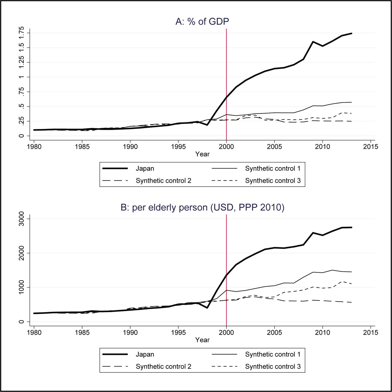
Figure 1
SC estimation for in-kind benefits for the elderly (% of GDP).
Notes: SC 1 is constructed from the original donor pool, SC 2 is constructed from the donor pool that excludes the country that receives the highest weights in the first SC estimation, and SC 3 is constructed from the donor pool that also excludes the country that receives the highest weights in the second SC estimation. Canada is excluded from the original donor pool due to lack of data. For SC estimation we use the synth command in Stata with the nested and allopt options. See Tables A4 and A5 in Appendix A3 for detailed estimation results.
SC 1 in the graph is constructed from the original donor pool and therefore its values are regarded as baseline counterfactual outcomes in the post-intervention period; that is, they represent the levels of in-kind benefits for the elderly if LTCI had not been introduced in Japan. As discussed in Section 3, SC estimates are the gaps between the outcomes of a treated unit and an SC. If an SC is validly constructed based on pre-intervention outcomes and predictors, SC estimates are expected to be around zero in the pre-intervention period and can be interpreted as causal effects in the post-intervention period.
SC 2 is constructed using SC estimation in which the country that receives the highest weight in the first SC estimation is excluded from the donor pool. SC 3 is constructed from a donor pool that additionally excludes the country that receives the highest weight in the second SC estimation. These robustness checks using SCs 2 and 3 are particularly important in our cross-country comparison, where there is a risk that some specific countries receive higher weights and idiosyncratic shocks in these countries may undermine the validity of the SC estimation. See also Abadie et al. (2015) for further discussion of this type of sensitivity checks. In Appendix A3, we provide the weights and the predetermined covariate values used for constructing SCs 1–3.
The results of SC estimation in Figure 1 indicate sharp increases in in-kind benefits for the elderly in Japan just after the introduction of LTCI. The gaps between the actual benefit level and those of the SCs persist and increase during the sample period and the size of the gaps reaches around one percentage point of GDP in panel A and about US$1,000 (in terms of PPP) in panel B in 2010, 10 years after LTCI introduction.
We argue that the expenditure increase by one percentage point of GDP within 10 years is not negligible and its aggregate-level impact on the social and economic outcomes such as female labor force participation is worth investigating.
5.2. Crowding out health expenditures?
We then examine whether LTCI introduction crowds out closely related public expenditure, that is, other public health expenditures. Figure 2 provides the results of SC estimation for public health expenditure. When we compare the actual outcomes with those of SCs 1–3 in panels A and B, the gaps between the outcomes in Japan and synthetic Japan are negative in the early 2000s, indicating that LTCI introduction might have led to the suppression of public health expenditure in this period. This suppression, however, appears to be small in terms of effect size, and we will further examine the significance of the observed suppression using placebo tests in Section 5.5. Overall, there is no clear evidence that LTCI introduction has caused a large public-expenditure shift from healthcare to LTC and the persistent suppression of public health expenditure.
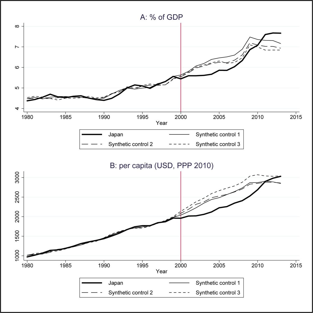
Figure 2
SC estimation of public health expenditure (% of GDP).
Notes: SC 1 is constructed from the original donor pool, SC 2 is constructed from a donor pool that excludes the country that receives the highest weights in the first SC estimation, and SC 3 is constructed from a donor pool that also excludes the country that receives the highest weights in the second SC estimation. Norway is excluded from the original donor pool due to a lack of data. For SC estimation, we use the synth command in Stata with the nested and allopt options. See Tables A6 and A7 in Appendix A3 for detailed estimation results.
5.3. Impacts on female labor force participation
Moving on from fiscal outcomes, Figure 3 provides our SC estimation results for female labor force participation (LFP) rates by age cohort. Despite the large fiscal expansion for LTCI, there is no sign of positive LTCI effects on the LFP rates in any of the cohorts. In fact, the female LFP rates for ages 50–54 and 55–59 appear to have been even suppressed after LTCI introduction, compared with those of all of the SCs.
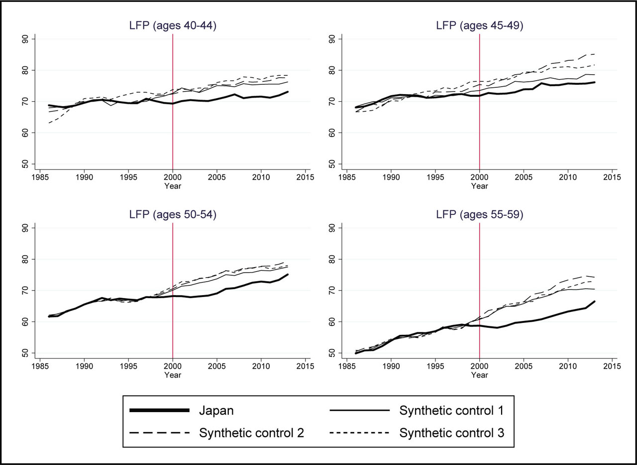
Figure 3
SC estimation of female LFP rates by age cohort.
Notes: See the note in Figure 1 for a detailed explanation of the graph. Due to data availability, the first year of our sample is 1986. Austria, Ireland, and Switzerland are excluded from the original donor pool due to lack of data. Except for the age cohort (55–59, lower right graph), Finland is also excluded due to lack of data. For SC estimation, we use the synth command in Stata with the nested and allopt options. See Tables A8–A11 in Appendix A3 for detailed estimation results.
The overall tendency of Japan's stagnated LFP rates in the post-intervention period suggests that there may exist a Japan-specific trend in the female LFP rates that is not taken into account by the SCs. This implies that SC estimates (i.e. outcome gaps between Japan and an SC) may not properly capture the causal effects of the LTCI introduction.
In order to eliminate this possible Japan-specific trend in the female LTF rates, we subtract the female LFP rate of ages 45–49 from the female LFP rate of ages 50–54 and ages 55–59 and then use these differenced variables as outcomes. The idea behind this procedure is that women aged 45–49, whose LFP rate is the highest among the four age cohorts in the post-reform period, are likely to be less affected by LTCI introduction, because their parents and parents-in-law tend to still have no need of LTC, whereas women aged 50–54 and 55–59 are likely to be more affected by the LTCI introduction because of a higher need for LTC for their parents or parents-in-law.
Thus, subtracting the female LFP rate of age cohort 45–49 from that of an older cohort may effectively eliminate the Japan-specific trend of female LFP, leaving a change in the older cohort LFP rate caused by LTCI introduction. This estimation strategy is akin to the triple-difference or difference-in-difference-in-difference (DDD) strategy, although we use the SC method after differencing the outcomes of “more affected” and “less affected” cohorts in both treated and control (or donor pool) countries.
The estimation results based on this strategy are shown in Figure 4. The left graph shows the trend of LFP-rate differences between the age cohorts 50–54 and 45–49 in Japan (bold solid lines) and its SCs. The right graph presents the counterpart trends of LFP-rate differences between the age cohorts 55–59 and 45–49. The results also do not indicate any positive impact of LTCI introduction on the female LFP rates for these two age cohorts. In fact, the right-hand graph again shows that the female LFP rates for the age cohort 55–59 seem to be suppressed after 2000 even after eliminating the trend of female LFP for the age cohort 45–49.
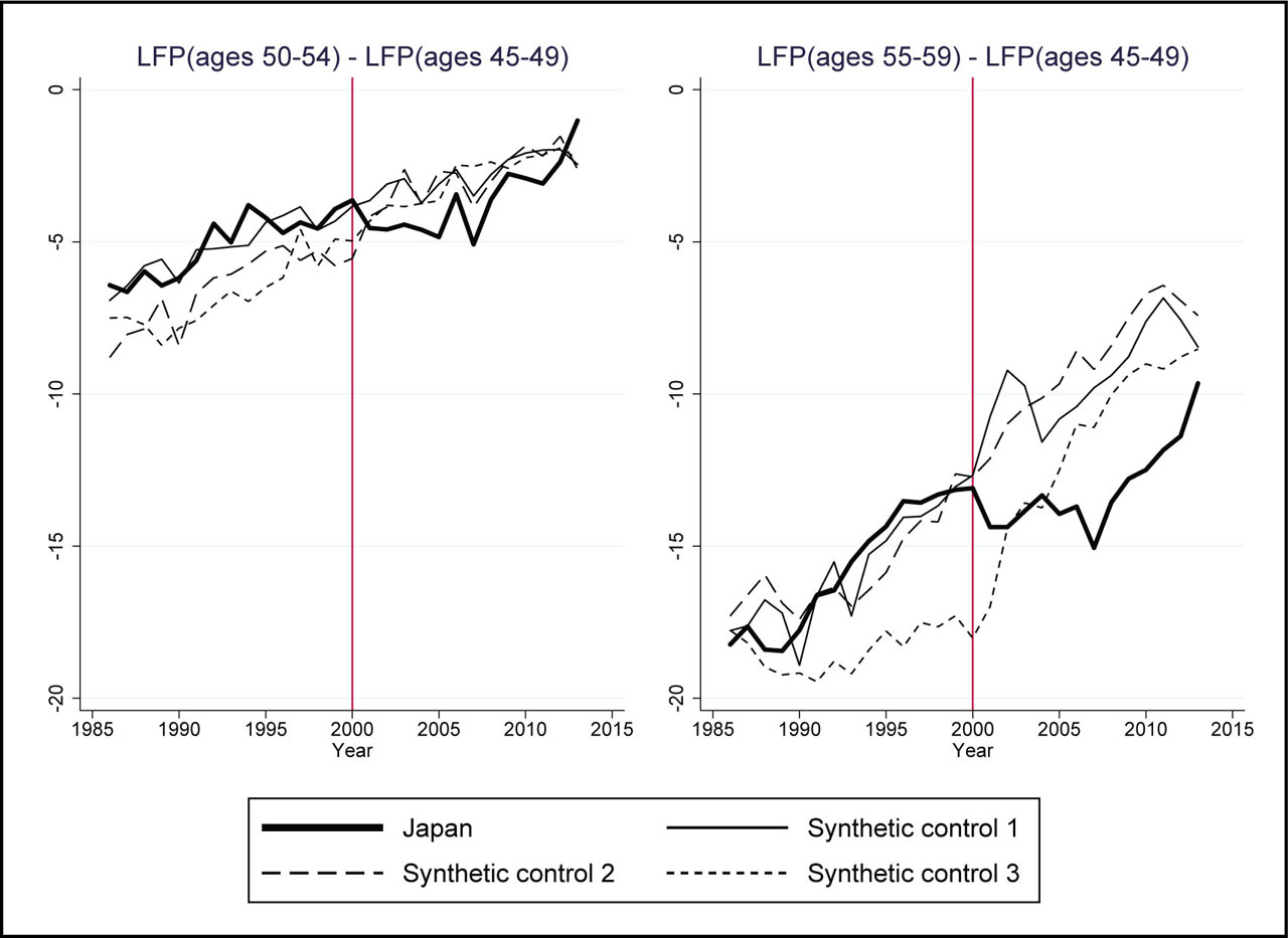
Figure 4
SC estimation for the difference in female LFP rates by age cohort.
Notes: See the note in Figure 1 for a detailed explanation of the graph. Due to data availability, the first year of our sample is 1986. Austria, Finland, Ireland, New Zealand, and Switzerland are excluded from the original donor pool due to lack of data. For SC estimation, we use the synth command in Stata with the nested and allopt options, but in cases in which there is an optimization error (due to a poor pre-intervention fit), we implement synth without nested and allopt. See Tables A12 and A13 in Appendix A3 for detailed estimation results.
5.4. Demeaned SC
To complement the above analyses, we also conduct additional SC estimation. That is, to alleviate imperfect pre-intervention fit, we implement SC estimation using demeaned outcomes in which pre-intervention outcome means are subtracted from outcome values (i.e. ). Ferman and Pinto (2019) shows that the demeaned SC estimator has better properties than the original SC estimator under some conditions, in particular when the imperfect pre-intervention fit exists in the conventional SC estimation. Note that we use only pre-intervention demeaned outcomes as predictors.
Figure 5 shows that the results of demeaned SC estimates are in line with those of the original estimates, while pre-intervention fits are improved for some LFP outcomes. Overall, we again find no sign of positive LTCI effects and female LFP rates for ages 55–59 (and possibly ages 50–54) appear to have been suppressed after LTCI introduction.
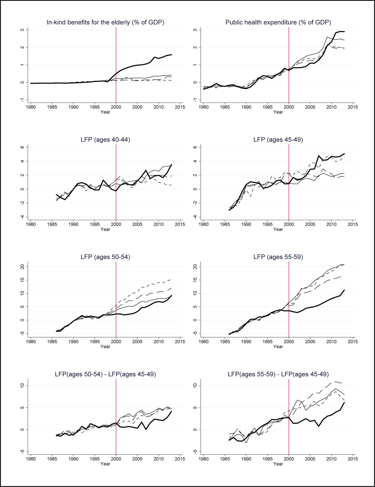
Figure 5
SC estimation of demeaned outcomes.
Notes: See the note and the legend in Figure 1 for detailed explanations of the graph. Due to data availability, the first year of our sample for the outcomes of female LFP rates is 1986. Due to lack of data, Canada is excluded from the donor pool for the outcome of in-kind benefits for the elderly, Norway for the outcome of public health expenditure, and Austria, Ireland, and Switzerland for the outcome of female LFP rates. Note that we use only pre-intervention demeaned outcomes as predictors. For SC estimation, we use the synth command in Stata with the nested and allopt options.
5.5. Placebo results
Figure 6 shows estimation results for placebo trials on all of the outcomes except for the results of demeaned SC estimation. On one hand, the first and second graphs in this figure indicate that the SC estimates for in-kind benefits for the elderly seem to be higher than most of the placebo estimates just after 2000, indicating that we can unambiguously conclude there was a fiscal impact of LTCI introduction (around a one percentage point increase in 2014). On the other hand, we do not find any clear effect on the public health expenditure, although negative SC estimates are relatively large around 2005 in particular, for per capita public health expenditure.
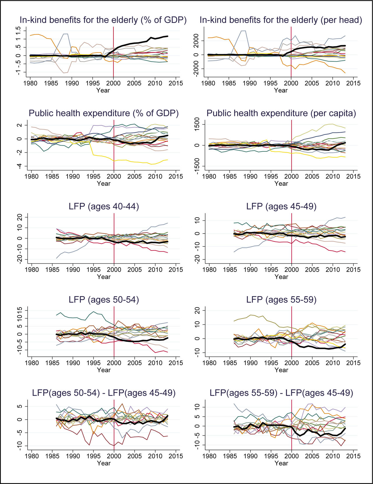
Figure 6
Placebo results.
Notes: Thick lines are Japan's SC estimates and the other lines are placebo SC estimates. We calculate placebo SC estimates by assigning the “label” of the intervention status to each control unit, using all the other control units as a donor pool. Note that the composition of donor pools (control units) is different depending on the outcome variables due to data constraints. For baseline SC estimates (bold black line), we use the synth command in Stata with the nested and allopt options. For placebo SC estimates (colored line), we implement synth without nested and allopt, because nested and allopt options sometimes result in optimization errors in some placebo trials.
Negative SC estimates for female LFP rates are sometimes clearly larger in size than most placebo estimates. In particular, the female LFP rate for ages 55–59 decreases after 2000 and the magnitude is larger than any placebo estimates. This tendency is mitigated if we subtract the female LFP for ages 45–49 from female LFP for ages 55–59 (the last two graphs). The last graph, nonetheless, indicates that the female LFP rate for ages 55–59 stagnated after 2000 and the magnitude is larger than most of the placebo estimates, although pre-intervention fits are poor for many placebo trials.
In the Appendices, we also provide the results of placebo tests for demeaned SC estimation (Appendix A4) and extended placebo tests based on permuted treatment assignment, resampled donor pools, and several test statistics (Appendix A5) to verity the above findings.
6. Further Analyses
This section discusses further SC analyses that address several concerns about our main SC estimation. We implement three different additional SC analyses. We briefly explain the backgrounds and results of these further examinations as follows.
First, we exclude from the donor pool the no-LTCI countries that experienced relatively high growth in in-kind benefits for the elderly in the post-intervention period. In the main SC estimation, we assume that Japan would have realized a similar level of in-kind benefits for the elderly to those of some no-LTCI countries if Japan had not introduced LTCI. However, if some control countries substantially increase their in-kind benefits for the elderly after 2000 without introducing LTCI, the interpretation of our SC estimation may be complicated, particularly if what we want to know is not the impact of LTCI itself but the impact of in-kind benefits for the elderly in general. We thus exclude several countries with the highest changes in in-kind benefits for the elderly in the 2000s (i.e., Austria, Finland, France, Spain, and the United Kingdom) based on Table A14 in Appendix A6. The SC estimation results do not change much from the baseline results, although the in-kind benefits for the elderly of SCs in the post-intervention period tend to be smaller than those in the baseline analysis (Figure A11 in Appendix A6).
Second, we remove five countries in which in-kind benefits for the elderly are relatively unreliable or unstable in the pre-intervention period. Specifically, we remove Italy, Belgium, and Portugal because their values of in-kind benefits for the elderly are zero in the period 1980–1989, possibly due to classification in OECD statistics, and we also drop Australia and Sweden because their in-kind benefits for the elderly fluctuate before the intervention years, probably due to their LTC reforms during this period (Cullen, 2003; Trydegård and Thorslund, 2010). Although it is not clear how these poor data properties in the pre-intervention period affect the post-intervention SC estimates, we implement SC estimation after excluding these five countries from the donor pool. The estimation results are again similar to our main findings (Figure A12 in Appendix A6).
Third, we implement in-time placebo SC estimation with a backdated intervention year. In the main analysis, the growth rate of the share of elderly in the pre-intervention period in Japan was larger than those of all the SCs (Appendix A3). Although it is not possible to solve this insufficient balancing on this variable using the standard SC method with positive weights, we can examine whether this insufficient balancing leads to serious estimation bias using in-time placebo tests proposed by Abadie et al. (2015) and Abadie (2019). To do this, we backdated the intervention period from 2000 to 1993 and implemented the in-time placebo test on a hold-out validation period to examine whether Japan's rapid population aging is a serious confounding factor in our analysis. The estimation results are shown in Figure A13 in Appendix A6. We neither observe an increase in in-kind benefits for the elderly nor stagnation of female LFP rates for ages 50–54 and 55–59, implying that the pre-LTCI rapid population aging in Japan was not a direct driving force of these outcomes. These results suggest that the sharp increase in the in-kind benefits for the elderly after 2000 in Japan and no counterpart increase in female LFP rates can be interpreted as evidence of no significant positive LTCI effect on female LFP.
7. Discussion and Conclusion
The nationwide LTCI introduction in Japan is one of the major social welfare reforms carried out in the 1990s and 2000s in aging OCED countries. In this paper, we investigate the impact of this LTCI introduction on fiscal outcomes and female labor force participation, exploiting the quasi-experimental features of LTCI introduction and using an SC method.
Our estimation results imply that LTCI introduction had a significant positive impact on the target expenditure item in Japan (i.e. in-kind benefits for the elderly), but we did not find robust effects on public health expenditure or female labor force participation rates. These results suggest that the LTCI program in Japan has not played a sufficient role to alter the family-dependent character of LTC provision and low female labor force participation in this country.
This macrolevel finding in our study may not be consistent with several recent microlevel studies that found some positive labor-supply effects of LTCI's in-kind benefits. Given the fact that we estimate the aggregate LTCI effects, whereas the previous studies study individual-level LTCI effects, we can provide several possible explanations that are consistent with both findings.
First of all, it is possible that we failed to detect some positive LTCI effects on female LFP rates because the power of our SC estimation may not be high enough. Even if this is the case, however, our analysis and several robustness checks still imply that an aggregate positive LTCI effect on female labor force participation, if it exists, is small enough to remain undetected by our analysis.
Second, LTCI benefits may have enabled more frail elderly people to live at home with their family. If this is the case, it is possible that some family caregivers worked more because of more in-kind benefits from LTCI (i.e. a positive effect), but some people worked less because they chose to be family caregivers for elderly people who would have been in hospitals or nursing homes if LTCI had not been introduced (i.e. a negative effect). Most individual-level studies focus on the first effect, but our aggregate-level study is meant to capture both effects.
This cancelling-out negative effect is at least somewhat plausible, given the fact that Japanese LTCI has mostly led to increases in residential care rather than institutional care. The ratio of the elderly who received residential LTCI services increased from 4.4% in 2000 to 12.4% in 2015. On the other hand, the total capacity of institutional care for the elderly (both public and private) only increased from 3.7% in 2000 to 5.5% in 2015. In addition, the number of long-term elderly inpatients (including social hospitalization) significantly decreased after the introduction of LTCI in 2000: the ratio of the elderly who were hospitalized for more than one month decreased from 2.5% in 1999 to 1.7% in 2014. These statistics imply that more old people who need health and social care now stay at home for a longer period using formal LTC services. This is exactly what the Japanese government intended to achieve through LTCI (Campbell and Ikegami, 2000, 2003), but this may increase the burden on some informal care-givers who would not have become caregivers if the elderly they take care of had instead been admitted to hospitals for a long period or stayed in nursing homes.
Overall, our study revealed that the Japanese LTCI introduction clearly boosted LTC spending but failed to boost labor force participation for middle-aged women. We discussed some possible mechanisms behind these results, but the mystery of no aggregate positive LTCI effect remains. Further studies are required to address this question and reconsider the potential roles of LTCI in female labor force participation.
Declarations
[3] Availability of Data and Materials
Data and materials generated and/or analyzed during the current study are available in the GitHub repository, https://github.com/michihito-ando/LongTermCare-IZA
[4] Conflicts of interest Competing Interests
The authors declare that they have no competing interests.
[5] Funding
This research is funded by a KAKENHI grants from the Japan Society for the Promotion of Science (grant number 15H03364, 17K03795, 18H00863).
[6] Contributed by Authors’ Contributions
MA designed the research idea, analyzed the data, and wrote the manuscript. MF refined the research idea, collected the data, and wrote the manuscript. YK refined the research design and revised the manuscript. All the authors read and approved the first manuscript. After YK passed away, MA and MF revised the manuscript and read and approved the final manuscript.
Acknowledgements
The authors are grateful to Emile Cammeraat, Peter H. Lindert, Masaru Sasaki, and to the conference and seminar participants at the FISS 2016 Conference, Keio University, JIPF 2016 Meeting, JEA 2017 Meeting, University of Toyama, IIPF 2018 Congress, GRIPS, and the University of Tokyo for their comments and suggestions. All errors are our own.
Appendix
A1
Comparisons of LTCI in Japan and Germany
Table A1
Institutional settings of LTCI programs in Germany and Japan, 2008 (Campbell et al., 2010)
| Germany | Japan | |
|---|---|---|
| Policy objective | Support family caregivers | Decrease burden of family caregivers |
| Policy design | Contain spending to within the premium level set by law | Increase expenditures as services become more available |
| Organized and managed | Sickness funds (but LTC is managed separately) | LTC insurance section of the municipal government or their coalitions |
| Financing | Premiums | Half by premiums, half by taxes |
| 1.95% of income up to a ceiling | 1/3 of premium revenue from those age 65+, with 6 premium levels based on income | |
| 2/3 from those ages 40–64 at 1% of income, up to a ceiling | ||
| Regional differences | No difference in premium levels | For those age 65+, premiums linked to local spending level |
| For those ages 40–64, pooled at national level and redistributed; municipalities having low income levels and more residents age 75+ receive more | ||
| Population covered | All ages | Unconditional for those age 65+ |
| Limited to age-related diseases for those ages 40–64 | ||
| Percentage of those age 65+ who are eligible | 10.50% | 17% |
| Percentage of those age 65+ who are receiving benefits | 10.5% (all of those eligible receive benefits) | 13.5% (20% of those eligible have not chosen to receive benefits) |
| Eligibility levels | Three (plus a limited additional hardship level in HCBS) | Two for the “preventive care” program, five for regular LTC insurance |
| Benefit ceilings per month ($ PPP) | No copayment or deductible | 10% copayment (included below) |
| Cash: $250–$794 plus caregiver pension premiums | Services only | |
| HCBS: $490–$1,730 (hardship: $2,260) | HCBS preventive care: $430–$950 | |
| Institutional care: $1,200–$1,730 | HCBS regular program: $1,440–$3,400 | |
| Room-and-board costs not covered; low income covered under public assistance | Institutional care: $1,680–$3,670 | |
| One-third of room-and-board costs covered, up to all costs paid by LTC insurance if income level is low | ||
| Fee schedule for services | Negotiated regionally between sickness funds and providers | Negotiated nationally, conversion factor for regional cost differences |
[i] Source: Exhibit 3 of Campbell et al. (2010). HCBS is home and community-based services.
Table A2
LTC spending on the elderly per person aged 65 and older (USD, PPP, 2005)
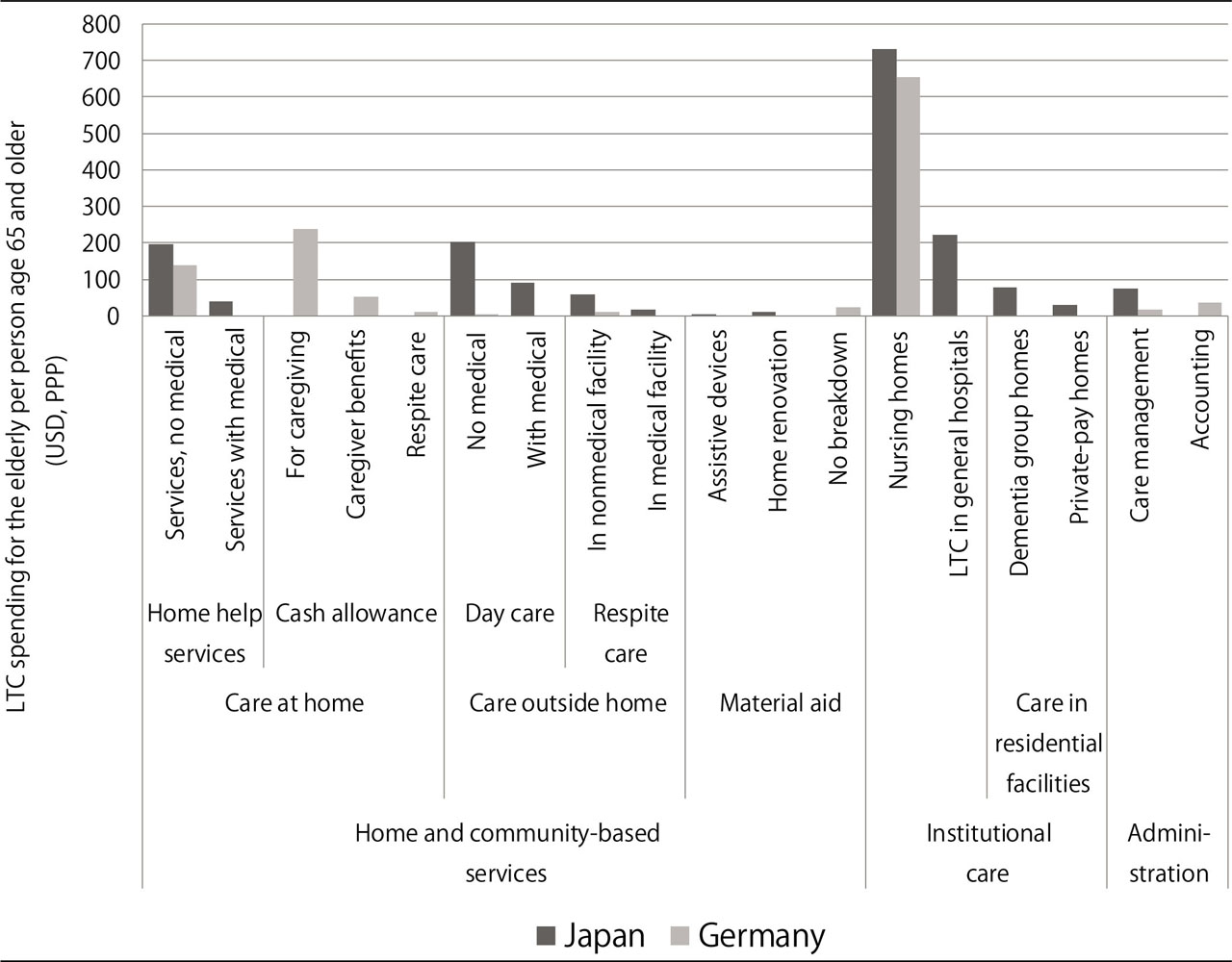
[i] Source: Exhibit 2 of Campbell et al., (2010).
A2
Variable Definitions and Sources
Table A3
Variable definitions and sources
| Outcomes (1980–2013) | Definition | Source |
|---|---|---|
| Public expenditure on benefits in kind for the elderly (% of GDP) | Public expenditure on benefits in kind for the elderly as percentages of GDP | OECD Database |
| Public expenditure on benefits in kind for the elderly (per elderly person) | Public expenditure on benefits in kind for the elderly per aged 65 and older, at constant prices (2010) and constant PPPs (2010) in USD | OECD Database |
| Total public expenditure on health care (% of GDP) | Total public expenditure on health care, as a percentage of GDP | OECD Database |
| Total public expenditure on health care (per capita) | Total public expenditure on health care per head, at constant prices (2010) and constant PPPs (2010) in USD | OECD Database |
| Female labour force participation rate by age cohort | Ratio of women in the labor force in an age cohort to the female population of the same age cohort | OECD Database |
| Predictors other than pre-intervention outcomes (1980–1999) | Definition | Source |
|---|---|---|
| Per capita real GDP | Expenditure-side real GDP (million US$, 2005, PPP) divided by population | PWT8.1 |
| Child population (%) | Population aged under 15 as % of population. | OECD Database |
| Elderly population (%) | Population aged 65 and older as % of population | OECD Database |
| Employment in agriculture (%) | Employment in agriculture as % of civilian employment | CWS |
| Employment in industry (%) | Employment in industry as % of civilian employment | CWS |
| Employment in services (%) | Employment in services as % of civilian employment | CWS |
| Annual growth rate of per capita real GDP (%) | Annual growth rate of per capita real GDP (%) | PWT8.1 |
| Annual growth rate of population (%) | Annual growth rate of population (%) | OECD Database |
| Annual growth rate of child population (%) | Annual growth rate of child population (%) | OECD Database |
| Annual growth rate of elderly population (%) | Annual growth rate of elderly population (%) | OECD Database |
[i] Notes: CWS and PWT 8.1 indicate “Comparative Welfare State Dataset” (Brady et al. (2014) and “Penn World Table 8.1” (Feenstra et al. (2015), respectively. Expenditure data based on the OECD database are from the OECD Social Expenditure Database (SOCX). Demographic data based on OECD databases are from the OECD Employment and Labour Force Statistics.
A3
Weights and Predictor Balance
Table A4
Outcome: in-kind benefits for the elderly (% of GDP)
| Weights | |||
|---|---|---|---|
| Country | Synthetic control 1 | Synthetic control 2 | Synthetic control 3 |
| Australia | 0.066 | 0.088 | 0.076 |
| Austria | 0.497 | - | - |
| Belgium | 0.155 | 0 | 0.515 |
| Denmark | 0 | 0 | 0.023 |
| Finland | 0 | 0 | 0 |
| France | 0 | 0 | 0 |
| Ireland | 0 | 0 | 0 |
| Italy | 0 | 0.489 | - |
| NewZealand | 0 | 0 | 0 |
| Norway | 0 | 0 | 0 |
| Portugal | 0 | 0.134 | 0.349 |
| Spain | 0.28 | 0 | 0 |
| Sweden | 0.002 | 0.037 | 0.037 |
| Switzerland | 0 | 0 | 0 |
| UnitedKingdom | 0 | 0.083 | 0 |
| UnitedStates | 0 | 0.169 | 0 |
| Predictor values | ||||
|---|---|---|---|---|
| Predictor | Treated | Synthetic control 1 | Synthetic control 2 | Synthetic control 3 |
| Lagged outcome (1980) | 0.101 | 0.108 | 0.101 | 0.099 |
| Lagged outcome (1981) | 0.104 | 0.108 | 0.101 | 0.102 |
| Lagged outcome (1982) | 0.110 | 0.108 | 0.098 | 0.102 |
| Lagged outcome (1983) | 0.110 | 0.108 | 0.095 | 0.101 |
| Lagged outcome (1984) | 0.109 | 0.108 | 0.094 | 0.097 |
| Lagged outcome (1985) | 0.109 | 0.108 | 0.090 | 0.099 |
| Lagged outcome (1986) | 0.122 | 0.106 | 0.089 | 0.099 |
| Lagged outcome (1987) | 0.115 | 0.130 | 0.124 | 0.131 |
| Lagged outcome (1988) | 0.114 | 0.132 | 0.133 | 0.136 |
| Lagged outcome (1989) | 0.120 | 0.132 | 0.130 | 0.138 |
| Lagged outcome (1990) | 0.127 | 0.162 | 0.163 | 0.161 |
| Lagged outcome (1991) | 0.138 | 0.170 | 0.176 | 0.170 |
| Lagged outcome (1992) | 0.153 | 0.162 | 0.191 | 0.187 |
| Lagged outcome (1993) | 0.167 | 0.169 | 0.204 | 0.197 |
| Lagged outcome (1994) | 0.182 | 0.187 | 0.204 | 0.195 |
| Lagged outcome (1995) | 0.214 | 0.200 | 0.204 | 0.217 |
| Lagged outcome (1996) | 0.221 | 0.227 | 0.213 | 0.229 |
| Lagged outcome (1997) | 0.241 | 0.225 | 0.220 | 0.221 |
| Lagged outcome (1998) | 0.186 | 0.275 | 0.278 | 0.279 |
| Lagged outcome (1999) | 0.431 | 0.288 | 0.262 | 0.269 |
| GDP per capita | 22.805 | 20.622 | 22.335 | 19.252 |
| Share of children (%) | 18.919 | 19.095 | 19.279 | 19.638 |
| Share of the elderly (%) | 12.294 | 14.261 | 14.092 | 14.207 |
| Share of agriculture (%) | 7.409 | 8.473 | 8.354 | 8.533 |
| Share of industry (%) | 34.082 | 33.070 | 31.543 | 30.437 |
| Share of service (%) | 58.509 | 58.439 | 60.079 | 61.009 |
| GDP per capita (growth rate) | 2.827 | 3.007 | 2.810 | 2.880 |
| Population (growth rate) | 0.436 | 0.387 | 0.429 | 0.306 |
| Share of children (growth rate) | −2.351 | −1.447 | −1.667 | −1.286 |
| Share of the elderly (growth rate) | 3.219 | 0.755 | 1.274 | 1.173 |
Table A5
Outcome: in-kind benefits for the elderly (per elderly person)
| Weights | |||
|---|---|---|---|
| Country | Synthetic control 1 | Synthetic control 2 | Synthetic control 3 |
| Australia | 0 | 0.043 | 0.01 |
| Austria | 0.591 | - | - |
| Belgium | 0 | 0 | 0.549 |
| Denmark | 0 | 0.027 | 0.034 |
| Finland | 0 | 0 | 0 |
| France | 0 | 0 | 0 |
| Ireland | 0 | 0 | 0 |
| Italy | 0 | 0.586 | - |
| NewZealand | 0 | 0 | 0 |
| Norway | 0.008 | 0.003 | 0.007 |
| Portugal | 0 | 0.148 | 0.137 |
| Spain | 0.4 | 0 | 0.233 |
| Sweden | 0 | 0.034 | 0.028 |
| Switzerland | 0 | 0 | 0.001 |
| UnitedKingdom | 0 | 0 | 0 |
| UnitedStates | 0 | 0.159 | 0 |
| Predictor values | ||||
|---|---|---|---|---|
| Predictor | Treated | Synthetic control 1 | Synthetic control 2 | Synthetic control 3 |
| Lagged outcome (1980) | 245.8 | 246.6 | 258.9 | 243.3 |
| Lagged outcome (1981) | 254.4 | 252.9 | 258.5 | 248.3 |
| Lagged outcome (1982) | 269.5 | 260.4 | 254.3 | 254.7 |
| Lagged outcome (1983) | 273.9 | 266.9 | 247.9 | 254.4 |
| Lagged outcome (1984) | 276.4 | 273.3 | 249.0 | 251.0 |
| Lagged outcome (1985) | 276.9 | 280.4 | 244.5 | 259.9 |
| Lagged outcome (1986) | 312.2 | 287.3 | 246.9 | 272.9 |
| Lagged outcome (1987) | 298.9 | 298.0 | 297.5 | 297.5 |
| Lagged outcome (1988) | 305.5 | 309.0 | 324.9 | 316.5 |
| Lagged outcome (1989) | 324.6 | 312.7 | 320.4 | 321.4 |
| Lagged outcome (1990) | 344.0 | 364.3 | 397.9 | 384.3 |
| Lagged outcome (1991) | 366.8 | 371.6 | 411.0 | 389.7 |
| Lagged outcome (1992) | 393.5 | 395.9 | 442.5 | 439.5 |
| Lagged outcome (1993) | 412.0 | 406.4 | 455.3 | 448.8 |
| Lagged outcome (1994) | 438.7 | 454.6 | 461.5 | 458.1 |
| Lagged outcome (1995) | 509.5 | 479.7 | 481.7 | 524.8 |
| Lagged outcome (1996) | 519.4 | 556.6 | 504.2 | 544.2 |
| Lagged outcome (1997) | 548.3 | 560.8 | 520.0 | 534.3 |
| Lagged outcome (1998) | 404.8 | 597.0 | 601.3 | 582.7 |
| Lagged outcome (1999) | 909.2 | 675.8 | 606.2 | 599.0 |
| GDP per capita | 22.805 | 19.628 | 22.131 | 19.639 |
| Share of children (%) | 18.919 | 19.002 | 18.900 | 19.252 |
| Share of the elderly (%) | 12.294 | 14.322 | 14.231 | 14.435 |
| Share of agriculture (%) | 7.409 | 10.037 | 9.210 | 7.436 |
| Share of industry (%) | 34.082 | 34.314 | 32.060 | 30.174 |
| Share of service (%) | 58.509 | 55.548 | 58.719 | 62.287 |
| GDP per capita (growth rate) | 2.827 | 3.204 | 2.829 | 2.653 |
| Population (growth rate) | 0.436 | 0.347 | 0.362 | 0.252 |
| Share of children (growth rate) | −2.351 | −1.695 | −1.857 | −1.423 |
| Share of the elderly (growth rate) | 3.219 | 0.778 | 1.364 | 1.174 |
Table A6
Outcome: public health expenditure (% of GDP)
| Weights | |||
|---|---|---|---|
| Country | Synthetic control 1 | Synthetic control 2 | Synthetic control 3 |
| Australia | 0.246 | 0.278 | - |
| Austria | 0 | 0 | 0 |
| Belgium | 0 | 0 | 0 |
| Canada | 0 | 0 | 0 |
| Denmark | 0.155 | 0.264 | 0.253 |
| Finland | 0 | 0 | 0 |
| France | 0.14 | 0.146 | 0.289 |
| Ireland | 0.05 | 0.11 | 0.09 |
| Italy | 0 | 0 | 0 |
| NewZealand | 0 | 0 | 0 |
| Portugal | 0.053 | 0.083 | 0.23 |
| Spain | 0 | 0 | 0 |
| Sweden | 0 | 0 | 0 |
| Switzerland | 0 | 0 | 0.123 |
| UnitedKingdom | 0.357 | - | - |
| UnitedStates | 0 | 0.118 | 0.016 |
| Predictor values | ||||
|---|---|---|---|---|
| Predictor | Treated | Synthetic control 1 | Synthetic control 2 | Synthetic control 3 |
| Lagged outcome (1980) | 4.374 | 4.480 | 4.477 | 4.533 |
| Lagged outcome (1981) | 4.438 | 4.543 | 4.484 | 4.599 |
| Lagged outcome (1982) | 4.548 | 4.467 | 4.487 | 4.555 |
| Lagged outcome (1983) | 4.695 | 4.552 | 4.488 | 4.487 |
| Lagged outcome (1984) | 4.566 | 4.587 | 4.528 | 4.413 |
| Lagged outcome (1985) | 4.527 | 4.586 | 4.571 | 4.506 |
| Lagged outcome (1986) | 4.593 | 4.556 | 4.555 | 4.501 |
| Lagged outcome (1987) | 4.619 | 4.542 | 4.554 | 4.520 |
| Lagged outcome (1988) | 4.510 | 4.499 | 4.538 | 4.594 |
| Lagged outcome (1989) | 4.434 | 4.437 | 4.484 | 4.511 |
| Lagged outcome (1990) | 4.396 | 4.500 | 4.542 | 4.558 |
| Lagged outcome (1991) | 4.495 | 4.706 | 4.726 | 4.722 |
| Lagged outcome (1992) | 4.707 | 4.881 | 4.822 | 4.807 |
| Lagged outcome (1993) | 4.999 | 5.013 | 4.992 | 5.056 |
| Lagged outcome (1994) | 5.147 | 4.944 | 4.947 | 4.984 |
| Lagged outcome (1995) | 5.098 | 4.994 | 5.105 | 5.119 |
| Lagged outcome (1996) | 4.982 | 5.024 | 5.134 | 5.194 |
| Lagged outcome (1997) | 5.180 | 5.217 | 5.130 | 5.149 |
| Lagged outcome (1998) | 5.314 | 5.301 | 5.153 | 5.150 |
| Lagged outcome (1999) | 5.560 | 5.562 | 5.448 | 5.420 |
| GDP per capita | 22.805 | 21.771 | 22.995 | 21.197 |
| Share of children (%) | 18.919 | 20.636 | 21.330 | 20.261 |
| Share of the elderly (%) | 12.294 | 13.853 | 12.914 | 13.982 |
| Share of agriculture (%) | 7.409 | 5.538 | 7.304 | 9.272 |
| Share of industry (%) | 34.082 | 28.957 | 27.643 | 30.068 |
| Share of service (%) | 58.509 | 65.539 | 64.878 | 60.761 |
| GDP per capita (growth rate) | 2.827 | 2.634 | 2.651 | 2.644 |
| Population (growth rate) | 0.436 | 0.539 | 0.697 | 0.384 |
| Share of children (growth rate) | −2.351 | −0.885 | −1.011 | −1.213 |
| Share of the elderly (growth rate) | 3.219 | 0.689 | 0.775 | 0.767 |
Table A7
Outcome: public health expenditure (per capita)
| Weights | |||
|---|---|---|---|
| Country | Synthetic control 1 | Synthetic control 2 | Synthetic control 3 |
| Australia | 0.303 | 0.313 | - |
| Austria | 0 | 0 | 0 |
| Belgium | 0 | 0 | 0 |
| Canada | 0 | 0.025 | 0.227 |
| Denmark | 0.031 | 0 | 0.065 |
| Finland | 0 | 0 | 0 |
| France | 0.095 | 0.09 | 0 |
| Ireland | 0 | 0 | 0 |
| Italy | 0 | 0 | 0 |
| NewZealand | 0 | 0.026 | 0 |
| Portugal | 0.002 | 0.189 | 0.278 |
| Spain | 0.323 | - | - |
| Sweden | 0 | 0 | 0 |
| Switzerland | 0.055 | 0.117 | 0.03 |
| UnitedKingdom | 0 | 0 | 0.169 |
| UnitedStates | 0.192 | 0.239 | 0.231 |
| Predictor values | ||||
|---|---|---|---|---|
| Predictor | Treated | Synthetic control 1 | Synthetic control 2 | Synthetic control 3 |
| Lagged outcome (1980) | 971.5 | 1012.0 | 1016.2 | 1011.5 |
| Lagged outcome (1981) | 1017.4 | 1031.6 | 1050.4 | 1060.0 |
| Lagged outcome (1982) | 1070.3 | 1044.4 | 1045.2 | 1079.2 |
| Lagged outcome (1983) | 1139.1 | 1119.5 | 1090.1 | 1106.8 |
| Lagged outcome (1984) | 1152.2 | 1168.3 | 1159.3 | 1123.9 |
| Lagged outcome (1985) | 1189.6 | 1191.1 | 1202.7 | 1175.7 |
| Lagged outcome (1986) | 1244.9 | 1226.9 | 1253.5 | 1227.1 |
| Lagged outcome (1987) | 1312.1 | 1276.7 | 1296.2 | 1274.8 |
| Lagged outcome (1988) | 1356.2 | 1340.8 | 1341.5 | 1336.5 |
| Lagged outcome (1989) | 1393.2 | 1395.3 | 1391.5 | 1372.4 |
| Lagged outcome (1990) | 1438.5 | 1458.7 | 1452.0 | 1461.5 |
| Lagged outcome (1991) | 1505.3 | 1529.2 | 1539.1 | 1559.8 |
| Lagged outcome (1992) | 1578.7 | 1613.3 | 1603.8 | 1622.4 |
| Lagged outcome (1993) | 1669.8 | 1670.6 | 1668.1 | 1679.8 |
| Lagged outcome (1994) | 1741.1 | 1712.4 | 1717.5 | 1705.3 |
| Lagged outcome (1995) | 1769.0 | 1735.9 | 1712.6 | 1709.3 |
| Lagged outcome (1996) | 1769.5 | 1782.3 | 1771.7 | 1756.6 |
| Lagged outcome (1997) | 1844.7 | 1831.8 | 1829.2 | 1831.5 |
| Lagged outcome (1998) | 1870.6 | 1890.5 | 1894.8 | 1906.1 |
| Lagged outcome (1999) | 1963.1 | 1983.6 | 1981.5 | 2000.0 |
| GDP per capita | 22.805 | 23.067 | 24.301 | 22.647 |
| Share of children (%) | 18.919 | 21.111 | 21.309 | 20.602 |
| Share of the elderly (%) | 12.294 | 12.691 | 12.430 | 13.094 |
| Share of agriculture (%) | 7.409 | 7.476 | 7.437 | 7.694 |
| Share of industry (%) | 34.082 | 28.452 | 28.306 | 29.255 |
| Share of service (%) | 58.509 | 64.091 | 64.074 | 63.051 |
| GDP per capita (growth rate) | 2.827 | 2.499 | 2.533 | 2.730 |
| Population (growth rate) | 0.436 | 0.807 | 0.896 | 0.650 |
| Share of children (growth rate) | −2.351 | −1.423 | −1.037 | −1.072 |
| Share of the elderly (growth rate) | 3.219 | 1.248 | 1.091 | 1.072 |
Table A8
Outcome: female labor force participation rate (ages 40–44)
| Weights | |||
|---|---|---|---|
| Country | Synthetic control 1 | Synthetic control 2 | Synthetic control 3 |
| Australia | 0.074 | 0 | 0.754 |
| Belgium | 0 | 0 | 0 |
| Canada | 0 | 0 | 0 |
| Denmark | 0 | 0 | 0 |
| France | 0 | 0 | 0 |
| Italy | 0.354 | 0.581 | - |
| NewZealand | 0.519 | - | - |
| Norway | 0 | 0 | 0 |
| Portugal | 0 | 0 | 0 |
| Spain | 0 | 0 | 0.103 |
| Sweden | 0.053 | 0.419 | 0 |
| UnitedKingdom | 0 | 0 | 0.143 |
| UnitedStates | 0 | 0 | 0 |
| Predictor values | ||||
|---|---|---|---|---|
| Predictor | Treated | Synthetic control 1 | Synthetic control 2 | Synthetic control 3 |
| Lagged outcome (1986) | 68.793 | 67.967 | 66.711 | 63.126 |
| Lagged outcome (1987) | 68.386 | 68.241 | 67.130 | 64.465 |
| Lagged outcome (1988) | 68.076 | 68.506 | 67.802 | 66.657 |
| Lagged outcome (1989) | 68.750 | 68.936 | 69.393 | 69.099 |
| Lagged outcome (1990) | 69.582 | 69.886 | 70.122 | 70.940 |
| Lagged outcome (1991) | 70.377 | 70.019 | 70.176 | 71.123 |
| Lagged outcome (1992) | 70.513 | 70.396 | 70.894 | 71.455 |
| Lagged outcome (1993) | 70.291 | 68.680 | 69.979 | 70.692 |
| Lagged outcome (1994) | 69.792 | 70.023 | 69.595 | 71.663 |
| Lagged outcome (1995) | 69.469 | 69.420 | 69.421 | 72.359 |
| Lagged outcome (1996) | 69.464 | 69.846 | 70.239 | 72.987 |
| Lagged outcome (1997) | 70.874 | 70.048 | 70.470 | 72.935 |
| Lagged outcome (1998) | 70.175 | 71.158 | 71.900 | 72.357 |
| Lagged outcome (1999) | 69.543 | 71.728 | 72.060 | 72.441 |
| GDP per capita | 25.479 | 22.040 | 23.947 | 24.747 |
| Share of children (%) | 17.315 | 20.248 | 16.895 | 21.091 |
| Share of the elderly (%) | 13.419 | 13.195 | 16.530 | 12.396 |
| Share of agriculture (%) | 6.511 | 8.505 | 6.021 | 5.403 |
| Share of industry (%) | 33.692 | 27.659 | 30.670 | 25.484 |
| Share of service (%) | 59.796 | 63.821 | 63.309 | 68.954 |
| GDP per capita (growth rate) | 4.126 | 3.151 | 3.413 | 3.273 |
| Population (growth rate) | 0.326 | 0.739 | 0.220 | 1.049 |
| Share of children (growth rate) | −2.637 | −1.090 | −1.185 | −0.974 |
| Share of the elderly (growth rate) | 3.521 | 1.383 | 1.335 | 1.277 |
Table A9
Outcome: female labor force participation rate (ages 45–49)
| Weights | |||
|---|---|---|---|
| Country | Synthetic control 1 | Synthetic control 2 | Synthetic control 3 |
| Australia | 0 | 0 | 0 |
| Belgium | 0 | 0 | 0.23 |
| Canada | 0 | 0 | 0 |
| Denmark | 0.157 | 0.315 | 0 |
| France | 0 | 0 | 0 |
| Italy | 0.378 | - | - |
| NewZealand | 0 | 0 | 0 |
| Norway | 0 | 0 | 0 |
| Portugal | 0.002 | 0 | 0 |
| Spain | 0 | 0.346 | - |
| Sweden | 0.327 | 0.338 | 0 |
| UnitedKingdom | 0 | 0 | 0.77 |
| UnitedStates | 0.136 | 0 | 0 |
| Predictor values | ||||
|---|---|---|---|---|
| Predictor | Treated | Synthetic control 1 | Synthetic control 2 | Synthetic control 3 |
| Lagged outcome (1986) | 68.095 | 68.345 | 66.704 | 66.679 |
| Lagged outcome (1987) | 68.445 | 69.243 | 68.221 | 66.829 |
| Lagged outcome (1988) | 69.318 | 69.972 | 69.176 | 67.203 |
| Lagged outcome (1989) | 70.652 | 69.846 | 68.560 | 68.895 |
| Lagged outcome (1990) | 71.711 | 71.180 | 70.682 | 70.238 |
| Lagged outcome (1991) | 72.120 | 71.292 | 70.978 | 70.137 |
| Lagged outcome (1992) | 72.009 | 71.608 | 71.323 | 72.161 |
| Lagged outcome (1993) | 71.915 | 71.521 | 72.215 | 72.580 |
| Lagged outcome (1994) | 71.197 | 71.091 | 71.393 | 73.261 |
| Lagged outcome (1995) | 71.319 | 71.973 | 73.068 | 73.384 |
| Lagged outcome (1996) | 71.609 | 71.872 | 73.026 | 74.470 |
| Lagged outcome (1997) | 72.243 | 71.866 | 73.184 | 73.988 |
| Lagged outcome (1998) | 72.374 | 72.282 | 73.227 | 74.962 |
| Lagged outcome (1999) | 71.816 | 73.243 | 74.415 | 76.385 |
| GDP per capita | 25.479 | 25.477 | 22.213 | 22.777 |
| Share of children (%) | 17.315 | 17.728 | 18.087 | 18.943 |
| Share of the elderly (%) | 13.419 | 15.843 | 15.726 | 15.664 |
| Share of agriculture (%) | 6.511 | 5.270 | 6.346 | 2.179 |
| Share of industry (%) | 33.692 | 29.198 | 28.755 | 29.087 |
| Share of service (%) | 59.796 | 65.533 | 64.799 | 68.734 |
| GDP per capita (growth rate) | 4.126 | 3.173 | 3.847 | 3.653 |
| Population (growth rate) | 0.326 | 0.367 | 0.328 | 0.264 |
| Share of children (growth rate) | −2.637 | −0.781 | −1.044 | −0.097 |
| Share of the elderly (growth rate) | 3.521 | 0.900 | 0.771 | 0.540 |
Table A10
Outcome: female labor force participation rate (ages 50–54)
| Weights | |||
|---|---|---|---|
| Country | Synthetic control 1 | Synthetic control 2 | Synthetic control 3 |
| Australia | 0 | 0 | 0 |
| Belgium | 0 | 0 | 0 |
| Canada | 0 | 0 | 0 |
| Denmark | 0.189 | 0.25 | 0.345 |
| France | 0 | 0 | 0 |
| Italy | 0.176 | 0.079 | 0.107 |
| NewZealand | 0 | 0 | 0 |
| Norway | 0 | 0 | 0.129 |
| Portugal | 0.191 | 0.163 | 0.199 |
| Spain | 0 | 0 | 0 |
| Sweden | 0.232 | - | - |
| UnitedKingdom | 0 | 0.461 | - |
| UnitedStates | 0.212 | 0.048 | 0.22 |
| Predictor values | ||||
|---|---|---|---|---|
| Predictor | Treated | Synthetic control 1 | Synthetic control 2 | Synthetic control 3 |
| Lagged outcome (1986) | 61.671 | 61.806 | 62.115 | 61.415 |
| Lagged outcome (1987) | 61.800 | 62.525 | 62.456 | 61.892 |
| Lagged outcome (1988) | 63.350 | 63.406 | 63.038 | 63.346 |
| Lagged outcome (1989) | 64.216 | 64.011 | 64.258 | 64.147 |
| Lagged outcome (1990) | 65.526 | 65.492 | 65.353 | 65.553 |
| Lagged outcome (1991) | 66.506 | 66.621 | 66.228 | 66.634 |
| Lagged outcome (1992) | 67.606 | 66.536 | 66.748 | 66.651 |
| Lagged outcome (1993) | 66.897 | 67.107 | 67.576 | 67.535 |
| Lagged outcome (1994) | 67.401 | 66.605 | 66.941 | 66.325 |
| Lagged outcome (1995) | 67.111 | 66.929 | 66.570 | 66.209 |
| Lagged outcome (1996) | 66.900 | 66.790 | 66.535 | 66.492 |
| Lagged outcome (1997) | 67.882 | 67.831 | 67.754 | 67.683 |
| Lagged outcome (1998) | 67.811 | 67.918 | 68.425 | 68.606 |
| Lagged outcome (1999) | 67.894 | 69.007 | 69.368 | 69.911 |
| GDP per capita | 25.479 | 24.429 | 22.430 | 24.880 |
| Share of children (%) | 17.315 | 18.642 | 18.672 | 18.848 |
| Share of the elderly (%) | 13.419 | 15.096 | 15.231 | 14.593 |
| Share of agriculture (%) | 6.511 | 6.663 | 5.489 | 6.994 |
| Share of industry (%) | 33.692 | 29.091 | 29.796 | 28.320 |
| Share of service (%) | 59.796 | 64.246 | 64.815 | 64.687 |
| GDP per capita (growth rate) | 4.126 | 3.580 | 3.817 | 3.491 |
| Population (growth rate) | 0.326 | 0.428 | 0.271 | 0.446 |
| Share of children (growth rate) | −2.637 | −0.838 | −0.588 | −0.758 |
| Share of the elderly (growth rate) | 3.521 | 0.861 | 0.651 | 0.676 |
Table A11
Outcome: female labor force participation rate (ages 55–59)
| Weights | |||
|---|---|---|---|
| Country | Synthetic control 1 | Synthetic control 2 | Synthetic control 3 |
| Australia | 0.16 | 0.473 | - |
| Belgium | 0 | 0 | 0 |
| Canada | 0 | 0 | 0.017 |
| Denmark | 0.047 | 0 | 0 |
| Finland | 0.15 | 0.198 | 0.291 |
| France | 0 | 0 | 0 |
| Italy | 0 | 0 | 0 |
| NewZealand | 0 | 0 | 0.12 |
| Norway | 0 | 0 | 0 |
| Portugal | 0.085 | 0 | 0.376 |
| Spain | 0 | 0 | 0 |
| Sweden | 0.094 | 0.329 | 0.196 |
| UnitedKingdom | 0 | 0 | 0 |
| UnitedStates | 0.464 | - | - |
| Predictor values | ||||
|---|---|---|---|---|
| Predictor | Treated | Synthetic control 1 | Synthetic control 2 | Synthetic control 3 |
| Lagged outcome (1986) | 49.863 | 50.187 | 50.489 | 50.848 |
| Lagged outcome (1987) | 50.806 | 50.640 | 51.522 | 50.685 |
| Lagged outcome (1988) | 50.919 | 51.550 | 52.017 | 52.105 |
| Lagged outcome (1989) | 52.208 | 52.932 | 52.897 | 53.244 |
| Lagged outcome (1990) | 53.944 | 54.066 | 54.152 | 54.459 |
| Lagged outcome (1991) | 55.500 | 54.725 | 54.979 | 55.372 |
| Lagged outcome (1992) | 55.556 | 55.269 | 54.811 | 55.271 |
| Lagged outcome (1993) | 56.404 | 55.283 | 55.097 | 54.865 |
| Lagged outcome (1994) | 56.359 | 56.602 | 55.988 | 55.646 |
| Lagged outcome (1995) | 56.965 | 57.053 | 56.945 | 56.623 |
| Lagged outcome (1996) | 58.088 | 57.869 | 58.617 | 58.233 |
| Lagged outcome (1997) | 58.670 | 57.949 | 57.486 | 57.383 |
| Lagged outcome (1998) | 59.070 | 58.635 | 58.121 | 57.892 |
| Lagged outcome (1999) | 58.667 | 59.958 | 59.529 | 60.042 |
| GDP per capita | 25.479 | 27.684 | 24.744 | 19.337 |
| Share of children (%) | 17.315 | 20.604 | 20.134 | 19.541 |
| Share of the elderly (%) | 13.419 | 13.281 | 13.950 | 14.310 |
| Share of agriculture (%) | 6.511 | 5.266 | 5.308 | 10.276 |
| Share of industry (%) | 33.692 | 26.479 | 25.959 | 29.771 |
| Share of service (%) | 59.796 | 68.222 | 68.634 | 59.953 |
| GDP per capita (growth rate) | 4.126 | 2.968 | 3.021 | 4.243 |
| Population (growth rate) | 0.326 | 0.858 | 0.830 | 0.389 |
| Share of children (growth rate) | −2.637 | −0.424 | −0.437 | −1.097 |
| Share of the elderly (growth rate) | 3.521 | 0.717 | 0.879 | 1.296 |
Table A12
Outcome: difference in female LFP rate (ages 50–54 and ages 45–49)
| Weights | |||
|---|---|---|---|
| Country | Synthetic control 1 | Synthetic control 2 | Synthetic control 3 |
| Australia | 0 | 0 | 0 |
| Belgium | 0 | 0 | 0 |
| Canada | 0 | 0 | 0 |
| Denmark | 0.189 | 0.25 | 0.345 |
| France | 0 | 0 | 0 |
| Italy | 0.176 | 0.079 | 0.107 |
| NewZealand | 0 | 0 | 0 |
| Norway | 0 | 0 | 0.129 |
| Portugal | 0.191 | 0.163 | 0.199 |
| Spain | 0 | 0 | 0 |
| Sweden | 0.232 | - | - |
| UnitedKingdom | 0 | 0.461 | - |
| UnitedStates | 0.212 | 0.048 | 0.22 |
| Predictor values | ||||
|---|---|---|---|---|
| Predictor | Treated | Synthetic control 1 | Synthetic control 2 | Synthetic control 3 |
| Lagged outcome (1986) | 61.671 | 61.806 | 62.115 | 61.415 |
| Lagged outcome (1987) | 61.800 | 62.525 | 62.456 | 61.892 |
| Lagged outcome (1988) | 63.350 | 63.406 | 63.038 | 63.346 |
| Lagged outcome (1989) | 64.216 | 64.011 | 64.258 | 64.147 |
| Lagged outcome (1990) | 65.526 | 65.492 | 65.353 | 65.553 |
| Lagged outcome (1991) | 66.506 | 66.621 | 66.228 | 66.634 |
| Lagged outcome (1992) | 67.606 | 66.536 | 66.748 | 66.651 |
| Lagged outcome (1993) | 66.897 | 67.107 | 67.576 | 67.535 |
| Lagged outcome (1994) | 67.401 | 66.605 | 66.941 | 66.325 |
| Lagged outcome (1995) | 67.111 | 66.929 | 66.570 | 66.209 |
| Lagged outcome (1996) | 66.900 | 66.790 | 66.535 | 66.492 |
| Lagged outcome (1997) | 67.882 | 67.831 | 67.754 | 67.683 |
| Lagged outcome (1998) | 67.811 | 67.918 | 68.425 | 68.606 |
| Lagged outcome (1999) | 67.894 | 69.007 | 69.368 | 69.911 |
| GDP per capita | 25.479 | 24.429 | 22.430 | 24.880 |
| Share of children (%) | 17.315 | 18.642 | 18.672 | 18.848 |
| Share of the elderly (%) | 13.419 | 15.096 | 15.231 | 14.593 |
| Share of agriculture (%) | 6.511 | 6.663 | 5.489 | 6.994 |
| Share of industry (%) | 33.692 | 29.091 | 29.796 | 28.320 |
| Share of service (%) | 59.796 | 64.246 | 64.815 | 64.687 |
| GDP per capita (growth rate) | 4.126 | 3.580 | 3.817 | 3.491 |
| Population (growth rate) | 0.326 | 0.428 | 0.271 | 0.446 |
| Share of children (growth rate) | −2.637 | −0.838 | −0.588 | −0.758 |
| Share of the elderly (growth rate) | 3.521 | 0.861 | 0.651 | 0.676 |
Table A13
Outcome: difference in female LFP rate (ages 55–59 and ages 45–49)
| Weights | |||
|---|---|---|---|
| Country | Synthetic control 1 | Synthetic control 2 | Synthetic control 3 |
| Australia | 0.16 | 0.473 | - |
| Belgium | 0 | 0 | 0 |
| Canada | 0 | 0 | 0.017 |
| Denmark | 0.047 | 0 | 0 |
| Finland | 0.15 | 0.198 | 0.291 |
| France | 0 | 0 | 0 |
| Italy | 0 | 0 | 0 |
| NewZealand | 0 | 0 | 0.12 |
| Norway | 0 | 0 | 0 |
| Portugal | 0.085 | 0 | 0.376 |
| Spain | 0 | 0 | 0 |
| Sweden | 0.094 | 0.329 | 0.196 |
| UnitedKingdom | 0 | 0 | 0 |
| UnitedStates | 0.464 | - | - |
| Predictor values | ||||
|---|---|---|---|---|
| Predictor | Treated | Synthetic control 1 | Synthetic control 2 | Synthetic control 3 |
| Lagged outcome (1986) | 49.863 | 50.187 | 50.489 | 50.848 |
| Lagged outcome (1987) | 50.806 | 50.640 | 51.522 | 50.685 |
| Lagged outcome (1988) | 50.919 | 51.550 | 52.017 | 52.105 |
| Lagged outcome (1989) | 52.208 | 52.932 | 52.897 | 53.244 |
| Lagged outcome (1990) | 53.944 | 54.066 | 54.152 | 54.459 |
| Lagged outcome (1991) | 55.500 | 54.725 | 54.979 | 55.372 |
| Lagged outcome (1992) | 55.556 | 55.269 | 54.811 | 55.271 |
| Lagged outcome (1993) | 56.404 | 55.283 | 55.097 | 54.865 |
| Lagged outcome (1994) | 56.359 | 56.602 | 55.988 | 55.646 |
| Lagged outcome (1995) | 56.965 | 57.053 | 56.945 | 56.623 |
| Lagged outcome (1996) | 58.088 | 57.869 | 58.617 | 58.233 |
| Lagged outcome (1997) | 58.670 | 57.949 | 57.486 | 57.383 |
| Lagged outcome (1998) | 59.070 | 58.635 | 58.121 | 57.892 |
| Lagged outcome (1999) | 58.667 | 59.958 | 59.529 | 60.042 |
| GDP per capita | 25.479 | 27.684 | 24.744 | 19.337 |
| Share of children (%) | 17.315 | 20.604 | 20.134 | 19.541 |
| Share of the elderly (%) | 13.419 | 13.281 | 13.950 | 14.310 |
| Share of agriculture (%) | 6.511 | 5.266 | 5.308 | 10.276 |
| Share of industry (%) | 33.692 | 26.479 | 25.959 | 29.771 |
| Share of service (%) | 59.796 | 68.222 | 68.634 | 59.953 |
| GDP per capita (growth rate) | 4.126 | 2.968 | 3.021 | 4.243 |
| Population (growth rate) | 0.326 | 0.858 | 0.830 | 0.389 |
| Share of children (growth rate) | −2.637 | −0.424 | −0.437 | −1.097 |
| Share of the elderly (growth rate) | 3.521 | 0.717 | 0.879 | 1.296 |
A4
Placebo Tests for Demeaned Outcomes
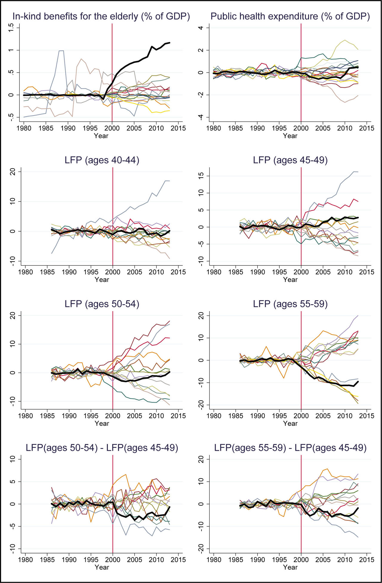
Figure A1
Placebo results for demeaned outcomes.
Notes: Thick lines are Japan's SC estimates and the other lines are placebo SC estimates. We calculate placebo SC estimates by assigning the “label” of the intervention status to each control unit, using all the other control units as a donor pool. Note that the composition of donor pools (control units) is different depending on the outcome variables due to data constraints. For baseline SC estimates (bold black line), we use the synth command in Stata with the nested and allopt options. For placebo SC estimates (colored line), we implement synth without nested and allopt, because nested and allopt options sometimes result in optimization errors in some placebo trials.
A5
Further Placebo Tests
A5.1. Motivation and setup
A limitation of the SC method is that this method does not provide formal statistical testing and the conventional placebo tests presented above are beneficial but still crude. In this section, based on the same parametric factor model used in Abadie et al. (2010), we first discuss how an SC estimate and counterpart placebo estimates can deviate from the true parameters of interest. We then provide four test statistics for extended placebo tests based on our discussion, placebo estimation Abadie et al. (2010), and leave-one-out estimation Abadie et al. (2015). Finally, we apply our proposed placebo tests to some selective outcomes.
Our extended placebo tests may be related to the emerging literature on the rigorous inference of SC methods (Doudchenko and Imbens, 2017; Ferman and Pinto, 2017; Firpo and Possebom, 2018; Chernozhukov et al., 2018), but we emphasize that they are still informal robustness/sensitivity checks.
We assume that the data-generating process in the absence of LTCI introduction can be expressed as the following “motivating model” in Abadie et al. (2010):
where Yit(Di) is the potential outcome defined in Section 3.3, δt is an unobserved time effect, Zi represents observed factor loadings (or predictors/covariates), μi indicates unobserved factor loadings, θt and λt are time-varying factors (or coefficients), and ɛit is unobserved transitory shocks with zero mean.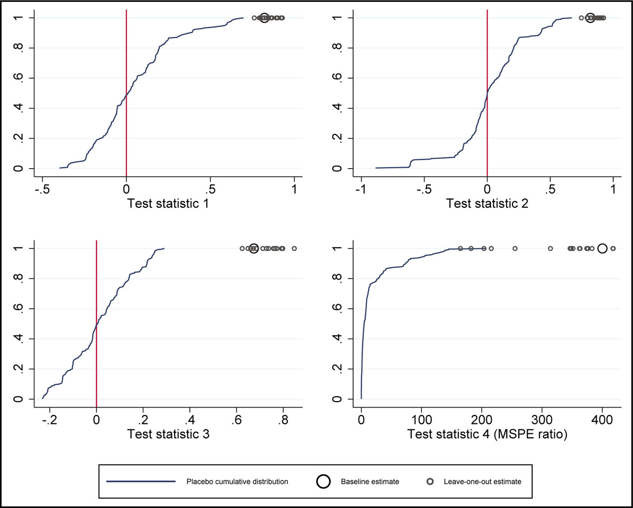
Figure A2
Extended placebo tests for in-kind benefits for the elderly (% of GDP).
Notes: The definitions of test statistics 1–4 are based on Eqs. (A.3) and (A.4). In each graph, the X-axis shows the values of test statistics and the Y-axis indicates the cumulative probability density of placebo-based test statistics. The large circle shows the value of a baseline test statistic for Japan and the small circles show the values of leave-one-out test statistics for Japan. Note that the nested and allopt options in the synth command in Stata are not used in all estimations, including baseline and leave-one-out estimations for Japan.
Based on Eqs. (2) and (A.1), we decompose the SC estimator as follows:
Equation (A.2) shows that an actual SC estimate can deviate from the true causal effect αit due to the following four components: First, the term represents a deviation that arises from the failure of observed predictor balancing. Second, captures a deviation caused by the failure of unobserved predictor balancing. Third, ɛit is by definition the unobserved transitory shocks for a treated unit (i.e. Japan) with zero mean. Fourth, is the negative of the weighted average of the unobserved transitory shocks for the control units.
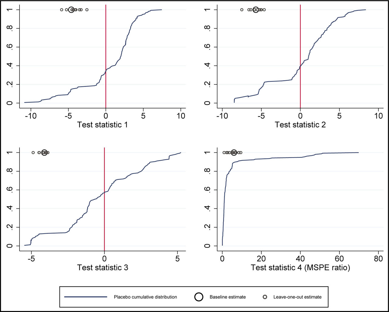
Figure A3
Extended placebo tests for the female LFP rate of ages 50–54.
Notes: The definitions of test statistics 1–4 are based on Eqs. (A.3) and (A.4). In each graph, the X-axis shows the values of test statistics and the Y-axis indicates the cumulative probability density of the placebo-based test statistics. The large circle shows the value of a baseline test statistic for Japan and the small circles show the values of leave-one-out test statistics for Japan. Note that the nested and allopt options in the synth command in Stata are not used in all estimations, including baseline and leave-one-out estimations for Japan.
Although Abadie et al. (2010) theoretically proved that the bias in the estimator of goes to zero as the number of re-intervention periods increases under the motivating model Eq. (A.1), there are several reasons why the above four deviations can persist in practice. First, the balance of observed and unobserved predictors, which make and zero under perfect balance, may not be sufficiently achieved due to lack of plausible control units in the donor pool. The problem of insufficient balance should not be overlooked in many comparative case studies where nonzero-weighted control units are often limited to somewhat similar but heterogeneous countries, states, regions, or municipalities. Second, the transitory shocks on the treated unit ɛit and the control units ɛkt can also cause the substantial deviation of from αit, because both ɛit and ɛkt are not averaged away in SC estimation: ɛit remains as it is due to a single treatment unit in a typical case study and the weights in are often assigned only to several control units in SC estimation.
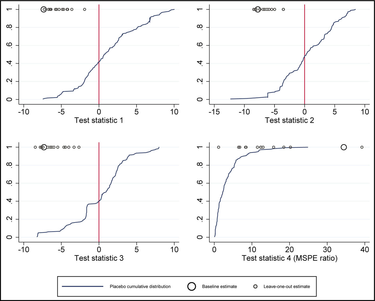
Figure A4
Extended placebo tests for the female LFP rate of ages 55–59.
Notes: The definitions of test statistics 1–4 are based on Eqs. (A.3) and (A.4). In each graph, the X-axis shows the values of test statistics and the Y-axis indicates the cumulative probability density of placebo-based test statistics. The large circle shows the value of a baseline test statistic for Japan and small circles show the values of leave-one-out test statistics for Japan. Note that the nested and allopt options in the synth command in Stata is not used in all estimations, including baseline and leave-one-out estimations for Japan.
Abadie et al. (2010)'s placebo test, which we also used in Section 5.5, can be interpreted as an informal test that investigates the distribution of the sum of the four deviations in Eq. (A.2). Assuming that the four deviations are unrelated to the intervention status Di, the sequential placebo assignment of the “label” of the treatment status to one of the control units is expected to generate the distribution of αit under the sharp null hypothesis of αit = 0. This distribution enables us to test whether the causal effect of αJt for the true treated unit i = J is plausibly nonzero.
An intuitive rationale for this placebo test is that if the absolute values of true SC estimates are larger than most placebo SC estimates, true SC estimates should reflect the causal effects of the intervention. Note, however, that this placebo test is clearly different from both the original Fisher's randomization inference (Fisher, 1937) and its extension to non-randomized observational studies (Rosenbaum, 1984; 2002; Ho and Imai, 2006) in the sense that we cannot argue that the “label” of treatment or intervention status is randomized in this placebo test, even after conditioning on covariates.
Abadie et al. (2015) provides another robustness check with “leave-one-out” SC estimation in which they exclude from the donor pool a control unit that receives a positive weight in a baseline SC estimation and then re-implement SC estimation. Because the exclusion of an important control unit may result in an increase in and as well as a change in in equation (A.2), the robustness of against this exclusion may support the plausibility of SC estimation. We have already implemented this type of robustness check in our baseline analysis in Section 5.
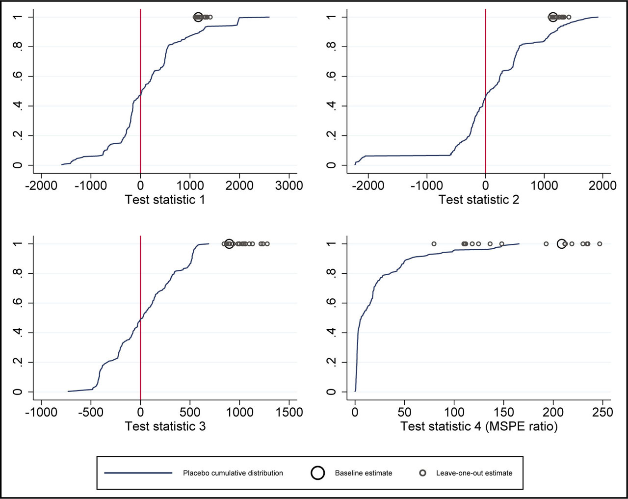
Figure A5
Extended placebo tests for in-kind benefits for the elderly per elderly person.
Note: see the note in Figure A2 for the estimation procedure.
In this section, in order to overcome the small number of placebo trials due to our small donor-pool size, we combine Abadie et al. (2010)'s placebo test and Abadie et al. (2015)'s robustness check by reassigning the treatment label to a control unit and resampling Nc − 1 control units from the original Nc control units in the donor pool. By combining both the placebo assignment and the “leave-one-out” procedure, we can obtain a richer distribution of the deviation terms in Eq. (A.2) under the sharp null hypothesis. Although this is still another informal placebo test, the number of placebo estimates in each t is Nc(Nc − 1), and this is much larger than the number of estimates in the original placebo test (i.e. Nc).
A5.2. Implementation
An actual placebo test is implemented as follows. First, we estimate baseline SC estimates for Japan (i = J), , and leave-one-out SC estimates for Japan, , where h is a control unit that is omitted from the donor pool. Second, we estimate leave-one-out placebo SC estimates for each control unit, in which we define , where i ≠ J indicates a control unit to which the placebo treatment is assigned. Note that the real treated units (i.e. Japan) are omitted from the donor pool in iterated placebo SC estimation for easier interpretation of the placebo estimates. Third, we compare the SC estimates and with the placebo SC estimates . For example, if most of and are above 95% or 97.5% of we may conclude that αJt is likely different from zero. On the other hand, if most of and are below 95% or 97.5% of , we conclude that αJt may not be different from zero. The threshold of 95% or 97.5% is based on the counterpart threshold of 90% or 95% significance level in normal two-sided tests. Note, however, that our placebo test is still informal as is the original.
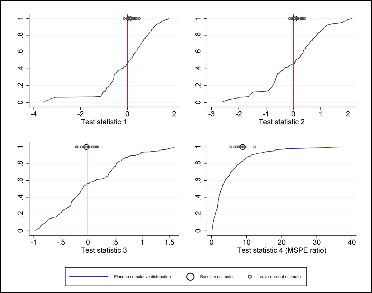
Figure A6
Extended placebo tests for public health expenditure (% of GDP).
Note: see the note in Figure A2 for the estimation procedure.
In practice, instead of using a placebo estimate (and baseline and leave-one-out estimates and ) in each year (t > T0), we use the following three placebo SC estimates (and their counterpart SC estimates) as test statistics in our placebo tests.
Test statistic 1 is the baseline statistic in which placebo SC estimates are simply averaged over post-intervention year s. Test statistic 2 is the gap between an average post-intervention SC estimate (i.e. test statistic 1) and an average pre-intervention SC estimate. An intuitive rationale for this test statistic is that the two deviation terms and in Eq. (A.2) should be similar between the pre and post-intervention periods if the coefficients θt and λt do not change much over time. If this is the case, subtracting the average pre-intervention SC estimate from the average post-intervention SC estimate may reduce some biases caused by insufficient balance in predictors. For example, if we assume that t = pre and post, αi, pre = 0, and θt and λt are constant over time, then .
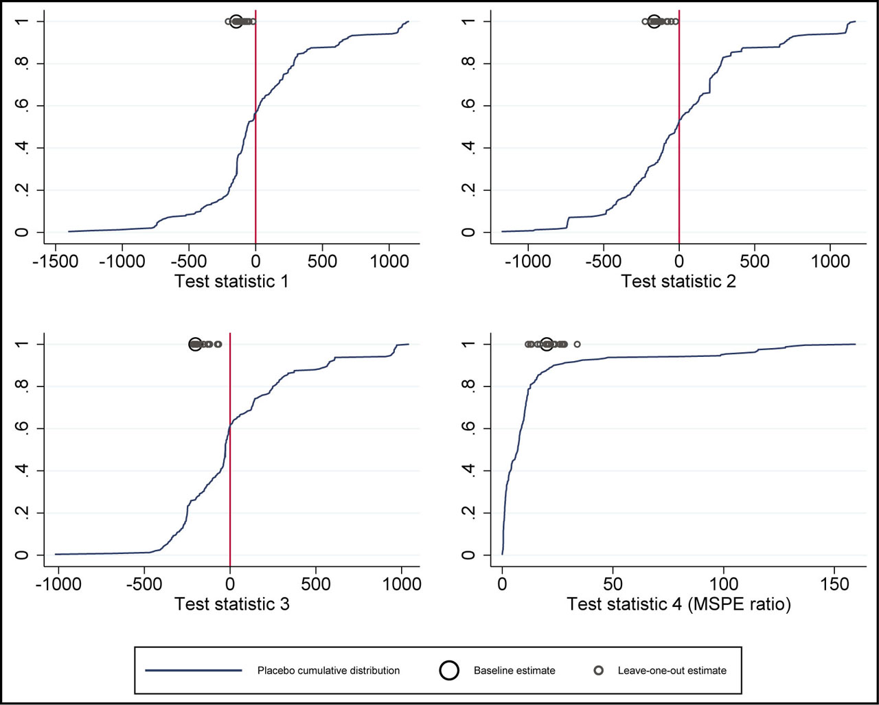
Figure A7
Extended placebo tests for public health expenditure per capita.
Note: see the note in Figure A2 for the estimation procedure.
The idea of test statistic 3 is similar to that of test statistic 2. In this statistic, the pre-intervention SC estimate at t = T0 is subtracted from test statistic 1 instead of subtracting the average pre-intervention estimate. This test statistic may be better than test statistic 2 in some cases, because SC estimates at t = T0 may reflect some bias (i.e. a poor pre-intervention fit) that arises just before the intervention and does not disappear after the intervention. In all three cases, we “test” the test statistics for Japan by comparing these values to placebo distributions based on Eq. (A.3).
Finally, Abadie et al. (2010) and subsequent studies use the post/pre-intervention ratios of MSPE (mean squared prediction error) to evaluate the SC estimates relative to their placebo counterparts. We also use the MSPE ratio of each placebo trial as an additional test statistic as:
A5.3. Results
Figure A2 shows the results of the extended placebo tests for in-kind benefits for the elderly as percentage of GDP. The distributions of the four test statistics based on Eqs. (A.3) and (A.4) are shown as cumulative distribution functions (CDFs) and the values of baseline and leave-one-out test statistics for Japan are presented as large and small circles, respectively. Note that nested and allopt options in synth command in Stata are not used in all estimations, including baseline and leave-one-out estimations for Japan, to avoid any optimization errors and to shorten the computation time.
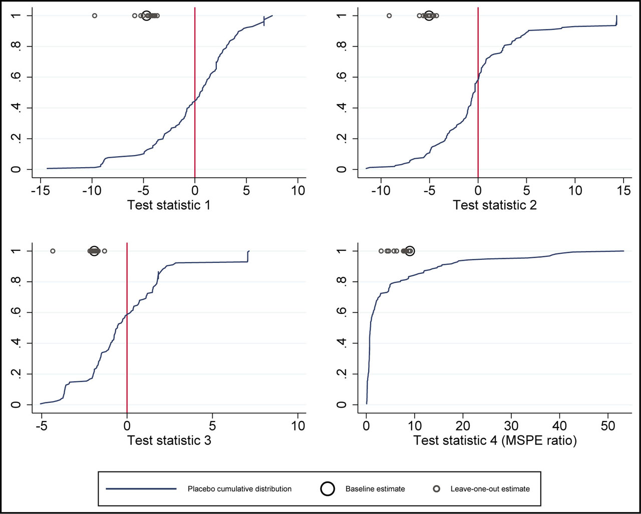
Figure A8
Extended placebo tests for Female labor force participation rate (ages 40–44).
Note: see the note in Figure A2 for the estimation procedure.
All the graphs in Figure A2 show that the baseline and leave-one-out test statistics for Japan are well above most of the placebo-based statistics. The first, second, and third graphs suggest that the baseline statistics and all leave-one-out test statistics for Japan are higher than any other placebo-based statistics. The last graph also shows that the post/pre-intervention MSPE ratios for baseline and leave-one-out SC estimates are higher than most placebo counterparts.
Figures A3 and A4 provide our extended placebo results for the female LFP rates of ages 50–54 and ages 55–59, respectively. Figure A3 shows that the values of test statistics for Japan are in the middle of the placebo-based test statistics, implying that they are not significantly different from the counterpart placebo-based test statistics. Figure A4 suggests that the baseline test statistics for Japan may be significantly different from the placebo-based test statistics, supporting the placebo result of the LFP rate for ages 55–59 in Figure 6. Leave-one-out test statistics for Japan are, however, unstable, implying that the baseline SC estimates are imprecise.
Finally, the placebo results for the other outcomes show that the values of Japan's baseline and most leave-one-out test statistics for these outcomes are not significantly different from the counterpart placebo-based test statistics, except for the outcome of in-kind benefits for the elderly per elderly person (Figures A5–A10).
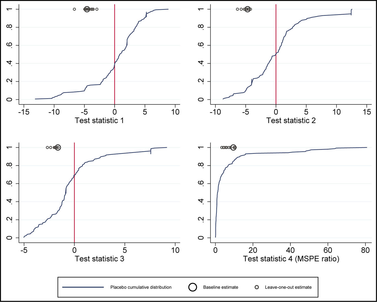
Figure A9
Extended placebo tests for female labor force participation rate (ages 45–49).
Note: see the note in Figure A2 for the estimation procedure.
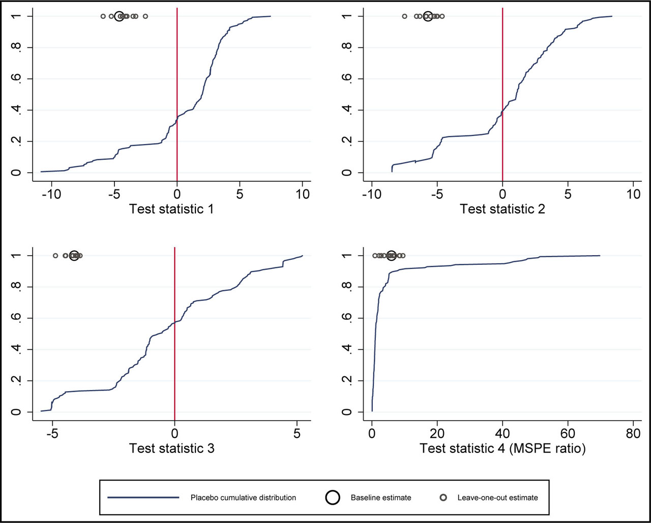
Figure A10
Extended placebo tests for female labor force participation rate (ages 50–54).
Note: see the note in Figure A2 for the estimation procedure.
Overall, our extended placebo tests indicate that there exist positive LTCI effects on in-kind LTC benefits for the elderly, but neither positive nor negative LTCI impacts on the female LFP rates are robustly observed. At the same time, our placebo tests also reveal the possibility that the female LFP rates for ages 55–59 stagnated after LTCI introduction, although we cannot confirm that LTCI introduction directly caused this stagnation.
A6
Further Analyses
A6.1. Further donor pool selections
Table A14
Changes in in-kind benefits for the elderly (% of GDP)
| Change in in-kind benefits for the elderly (% of GDP) | |||
|---|---|---|---|
| Country | 1999–2005 (% point) | Country | 1999–2010 (% point) |
| Japan | 0.713 | Japan | 1.096 |
| Netherlands | 0.243 | Spain | 0.469 |
| Spain | 0.183 | Finland | 0.354 |
| United Kingdom | 0.160 | Netherlands | 0.343 |
| Finland | 0.152 | France | 0.261 |
| France | 0.148 | Austria | 0.216 |
| Austria | 0.108 | United Kingdom | 0.158 |
| Australia | 0.043 | Denmark | 0.129 |
| Denmark | 0.035 | Switzerland | 0.081 |
| Portugal | 0.013 | Belgium | 0.079 |
| Switzerland | 0.010 | Portugal | 0.061 |
| Italy | 0.004 | Italy | 0.033 |
| Germany | 0.002 | Germany | 0.007 |
| United States | 0.000 | New Zealand | −0.001 |
| New Zealand | −0.001 | Ireland | −0.009 |
| Belgium | −0.016 | United States | −0.010 |
| Sweden | −0.067 | Sweden | −0.104 |
| Ireland | −0.110 | Norway | −0.192 |
| Norway | −0.410 | Australia | −0.444 |
[i] Notes: Calculated by the authors based on OECD Database. See also Table A3 in Appendix A2 for the definition of in-kind benefits for the elderly (% of GDP).
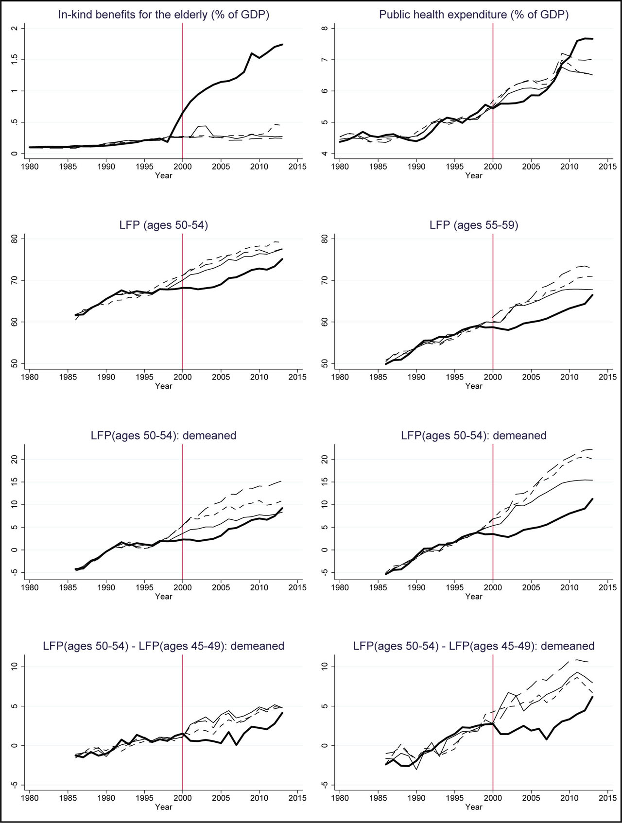
Figure A11
SC estimation with limited donor pool countries 1.
Notes: See the note and the legend in Figure 1 for detailed explanations of the graph. Due to data availability, the first year of our sample for the outcome of female LFPs is 1986. Countries with relatively high growth in the in-kind benefits for the elderly in the periods 1999–2005 or 1999–2010 (i.e., Austria, Finland, France, Spain, and the United Kingdom) are excluded from the donor pool. In addition, due to lack of data, Canada is excluded from the donor pool for the outcome of in-kind benefit for the elderly, Norway for the outcome of public health expenditure, and Ireland and Switzerland for the outcome of female LFP rates. For SC estimation, we use the synth command in Stata with the nested and allopt options.
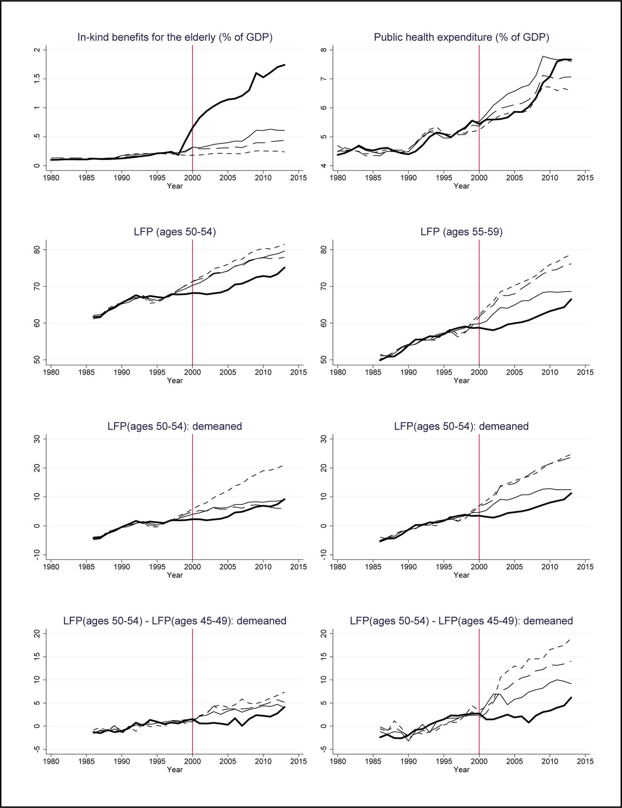
Figure A12
SC estimation with limited donor pool countries 2.
Notes: See the note and the legend in Figure 1 for detailed explanations of the graph. Due to data availability, the first year of our sample for the outcome of female LFP rates is 1986. Italy, Belgium, and Portugal are excluded from the donor pool due to zero values of in-kind benefits for the elderly in the period 1980–1989 and Australia and Sweden are also dropped from the donor pool because of fluctuating values in in-kind benefits for the elderly in the pre-intervention period. In addition, due to lack of data, Canada is excluded from the donor pool for the outcome of in-kind benefit for the elderly, Norway for the outcome of public health expenditure, and Austria, Ireland, and Switzerland for the outcome of female LFP rates. For SC estimation, we use the synth command in Stata with the nested and allopt options.
A6.2. In-time placebo analysis
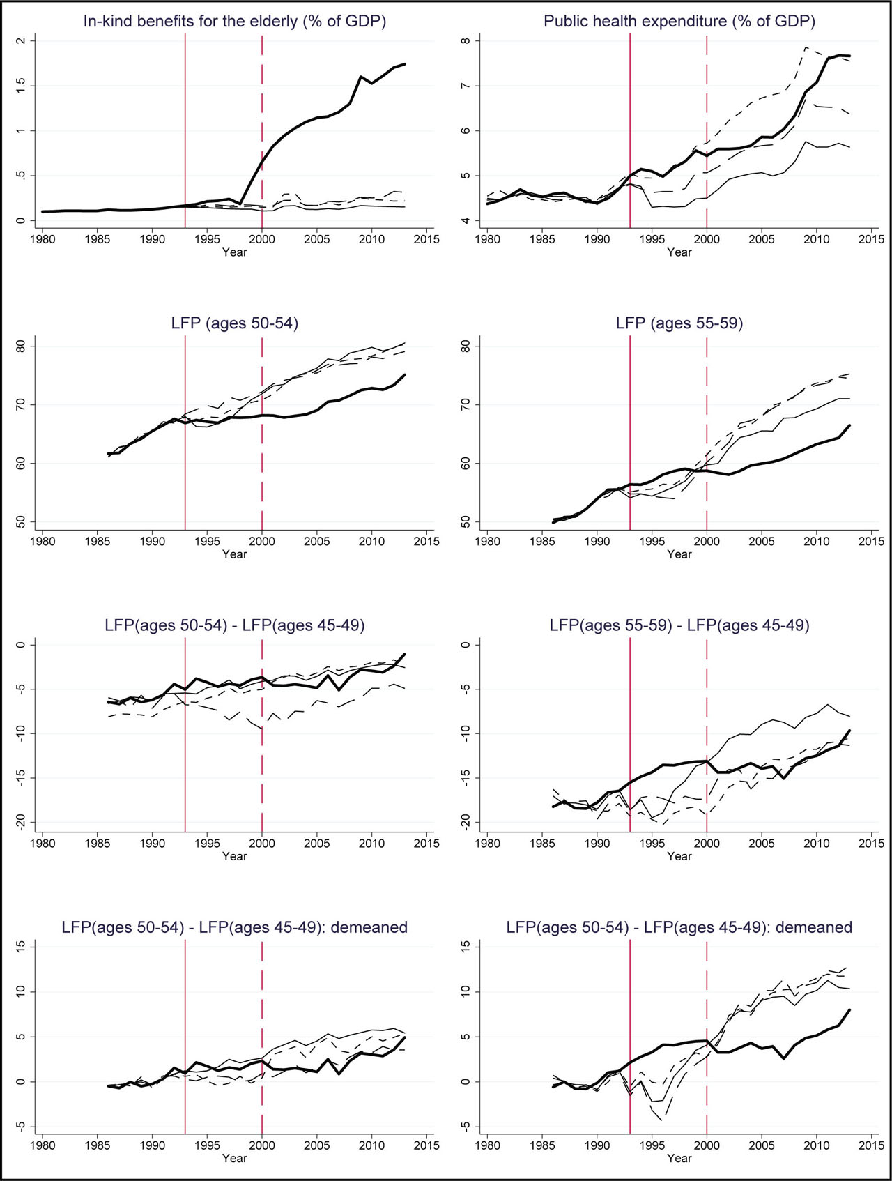
Figure A13
In-time placebo SC estimation with a backdated intervention year.
Notes: See the note and the legend in Figure 1 for detailed explanations of the graph. Due to data availability, the first year of our sample for the outcome of female LFP is 1986. In this SC estimation, the backdated intervention year is set as 1993 (solid vertical line) and therefore the period 1993–1999 is interpreted as the in-time placebo period. Due to lack of data, Canada is excluded from the donor pool for the outcome of in-kind benefit for the elderly, Norway for the outcome of public health expenditure, and Austria, Ireland, and Switzerland for the outcome of female LFP rates. For SC estimation, we use the synth command in Stata with the nested and allopt options.