
Figure 1
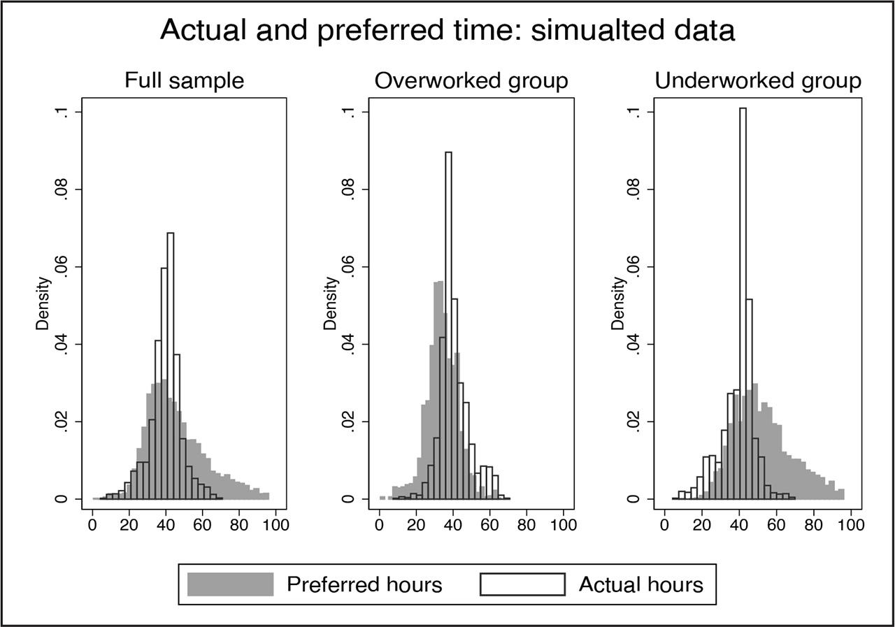
Figure 2
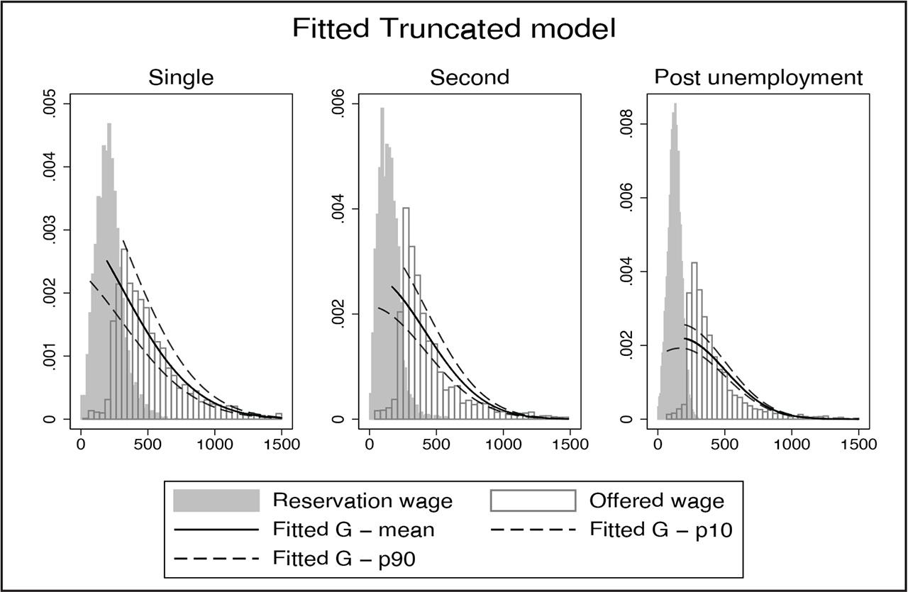
Figure 3
Figure 4
Figure 5
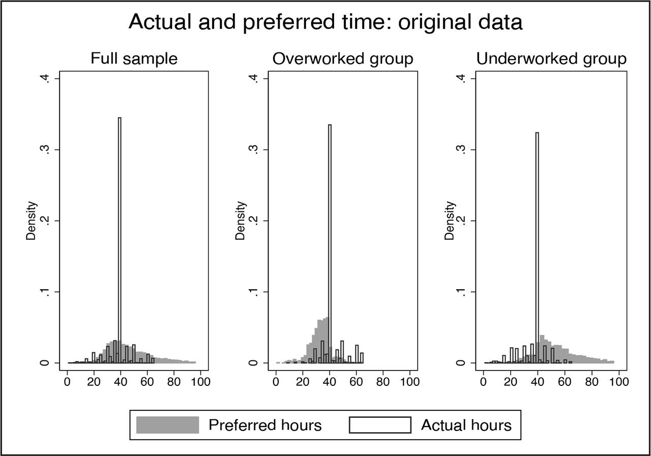
Figure 6
Estimated conditional reservation wages (cent)_ The proportion of observed accepted wages w′ smaller than the estimated ξ (percent)_ Estimated offer acceptance rates for single job offers, second job offers, and post-unemployment offers_
| q | 0.2 | 0.5 | 1 | 2 | 3 | 5 |
|---|---|---|---|---|---|---|
| Estimated conditional reservation wages,
| 57 | 82 | 113 | 158 | 191 | 231 |
| Pr(w′ < ξ) - in percent | 0.6 | 0.7 | 1.0 | 1.6 | 2.3 | 3.4 |
| Acceptance probability of single job offers,
| 0.89 | 0.87 | 0.78 | 0.61 | 0.41 | 0.20 |
| Acceptance probability of second job offers,
| 0.86 | 0.84 | 0.76 | 0.60 | 0.53 | 0.24 |
| Acceptance probability of post-unemployment offers,
| 0.93 | 0.90 | 0.85 | 0.72 | 0.54 | 0.20 |
Observed offered wages and estimated conditional reservation wages for different types of job, measured in cent q = 2_
| Job types | Observed offered wage | Estimated reservation wage | ||||
|---|---|---|---|---|---|---|
| Single | Second | Post-unemployment | Single | Second | Post-unemployment | |
| Mean | 517 | 434 | 408 | 218 | 154 | 125 |
| Median | 446 | 355 | 338 | 206 | 139 | 124 |
| S.D. | 268 | 239 | 212 | 121 | 113 | 53 |
Estimated values of leisure a (cent), actual working hours h (weekly hours), estimated optimal working hours h1* h_1^* (weekly hour), and their difference Δh_ Different values of q used in quantile regression_
| a |
| Δh |
| overworked group | underworked group | |||||
|---|---|---|---|---|---|---|---|---|---|---|
| h1 |
| Δh | h1 |
| Δh | |||||
| q = 0.2 | 1595 | 46.6 | −7.6 | 0.36 | 41.7 | 32.4 | 9.3 | 37.5 | 54.7 | −17.2 |
| q = 0.5 | 1655 | 46.6 | −7.6 | 0.36 | 41.7 | 32.9 | 8.8 | 37.5 | 54.6 | −17.1 |
| q = 1 | 1655 | 46.8 | −7.8 | 0.36 | 41.7 | 32.6 | 9.1 | 37.5 | 54.7 | −17.2 |
| q = 2 | 1680 | 46.5 | −7.5 | 0.37 | 41.5 | 33.1 | 8.5 | 37.5 | 54.4 | −16.9 |
| q = 3 | 1681 | 47.5 | −8.7 | 0.34 | 41.2 | 33.5 | 7.8 | 37.5 | 54.8 | −17.2 |
| q = 5 | 1693 | 48.0 | −9.2 | 0.34 | 41.1 | 33.8 | 7.3 | 37.5 | 55.2 | −17.7 |
Estimated value of leisure a (cent), wage elasticity of optimal leisure time ɛl,w1 and ɛl,w2, actual working hours h1 (weekly hour), estimated optimal hours h1* h_1^* (weekly hour), working hours mismatches Δh=h1−h1* \Delta h = {h_1} - h_1^* (weekly hour)_ q = 2_ Dierent values of e˜i {\tilde e_i} _
| a | ɛl,w1 | ɛl,w2 | h1 |
| Δh |
| overwork | underwork | |
|---|---|---|---|---|---|---|---|---|---|
| Δh | Δh | ||||||||
|
| 1680 | −0.26 | −0.40 | 39.0 | 46.5 | 8.5 | −16.9 | ||
|
| 1508 | −0.28 | −0.51 | 39.0 | 42.1 | 9.0 | −13.7 | ||
|
| 1485 | −0.32 | −0.59 | 39.0 | 38.3 | 0.6 | 0.53 | 9.9 | −10.1 |
Descriptive statistics_
| Variables | Mean | SD | min | max |
|---|---|---|---|---|
| Real wage (cent) in current job | 452 | 261 | 1 | 1858 |
| Real wage (cent) in new single job offer | 517 | 267 | 9 | 1636 |
| Real wage (cent) in new second job offer | 434 | 239 | 39 | 1623 |
| Real wage (cent) in post unemployment job offer | 409 | 212 | 67 | 1644 |
| Weekly working hours in current job (one job) | 36.6 | 11.7 | 0 | 168 |
| Weekly working hours in current jobs (two jobs) | 62.1 | 19.5 | 0 | 168 |
| Weekly working hours in new single job | 39.1 | 8.77 | 1 | 168 |
| Weekly working hours in new second job | 29.8 | 13.7 | 1 | 140 |
| Weekly working hours in post unemployment job | 35.0 | 11.0 | 1 | 144 |
| Weekly leisure hours | 127 | 16.0 | 0 | 168 |
| Duration (week) for employment spell (one job) | 106 | 133 | 1 | 1346 |
| Duration (week) for employment spell (two jobs) | 34.2 | 47.1 | 1 | 630 |
| Duration (week) for unemployment spell | 49.5 | 65.6 | 1 | 631 |
| Previous work experience (week) | 391 | 197 | 1 | 1646 |
| Number of jobs held prior to change in job status | 7.25 | 4.67 | 1 | 36 |
| Age | 29.2 | 3.13 | 25 | 35 |
| Female (dummy) | 0.50 | 0.50 | 0 | 1 |
| White (dummy) | 0.51 | 0.50 | 0 | 1 |
| Black (dummy) | 0.28 | 0.45 | 0 | 1 |
| Married (dummy) | 0.32 | 0.47 | 0 | 1 |
| Parenthood (dummy) | 0.72 | 0.45 | 0 | 4 |
| Net worth (thousand dollars) | 61 | 136 | −300 | 600 |
| Non high school qualification or lower (dummy) | 0.15 | 0.35 | 0 | 1 |
| Industry - public sector (dummy) | 0.22 | 0.41 | 0 | 1 |
| Industry- professional services (dummy) | 0.21 | 0.41 | 0 | 1 |
| Real interest rate (percent) | 1.80 | 1.90 | 0.50 | 6.02 |
Estimated job offer rates λj, separation rates δj, and acceptance rates Pj in percent_
| Job types | Job offer rates, λj | Job separation rates, δj | Job acceptance rates, Pj | |||||
|---|---|---|---|---|---|---|---|---|
| Single | Second | Post-unemp | Job 1 | Job 2 | Single | Second | Post-unemp | |
| Mean | 0.78 | 0.55 | 2.18 | 1.24 | 1.71 | 61.0 | 59.8 | 72.4 |
| 1 percentile | 0.18 | 0.10 | 1.16 | 0.14 | 0.40 | 5.58 | 7.02 | 21.6 |
| 99 percentile | 7.36 | 5.86 | 7.62 | 14.1 | 5.31 | 98.9 | 98.9 | 99.7 |
Wage rate w1 (cent), estimated value of leisure a (cent), adjustment factor B and E, wage elasticity of optimal leisure time ɛl,w1 and ɛl,w2, actual working hours h1 (weekly hour), estimated optimal working hours h1* h_1^* (weekly hour), and the difference between h1 and h1* h_1^* (weekly hour)_
| w1 | a | B | E | ɛl,w1 | ɛl,w2 | h1 |
|
| |
|---|---|---|---|---|---|---|---|---|---|
| Mean | 445 | 1680 | 1.02 | 0.67 | −0.26 | −0.40 | 39.0 | 46.5 | −7.50 |
| S.D. | 239 | 410 | 0.01 | 0.11 | 0.12 | 0.22 | 8.39 | 17.4 | 17.7 |
| 1 percentile | 126 | 1101 | 1.00 | 0.40 | −0.71 | −1.27 | 12 | 14.4 | −57.9 |
| 99 percentile | 1345 | 3152 | 1.08 | 0.92 | −0.08 | −0.10 | 65 | 97.1 | 27.7 |
Actual working hours h1 (weekly hour), estimated optimal hours h1* h_1^* (weekly hour), Δh=h1−h1* \Delta h = {h_1} - h_1^* (weekly hour)_ q = 2_ Different SD_
| h1 |
| Δh |
| overwork group | underwork group | |||||
|---|---|---|---|---|---|---|---|---|---|---|
| h1 |
| Δh | h1 |
| Δh | |||||
| SD = 0 | 39.0 | 46.5 | −7.5 | 0.37 | 41.5 | 33.1 | 8.5 | 37.5 | 54.4 | −16.9 |
| SD = 2 | 39.8 | 46.5 | −7.1 | 0.37 | 40.5 | 33.3 | 7.2 | 38.8 | 54.3 | −15.6 |
| SD = 4 | 39.8 | 46.5 | −6.7 | 0.38 | 40.5 | 34.0 | 6.4 | 39.4 | 54.0 | −14.5 |
| SD = 8 | 40.7 | 46.5 | −5.8 | 0.38 | 42.8 | 36.2 | 6.6 | 39.3 | 52.8 | −13.5 |
Estimated parameter for the value of leisure (measured in e−6), the estimated partial effect ai2αk a_i^2{\alpha _k} - mean, minimum and maximum (measured in cent)_
| Variables | αk | The partial effect
| ||
|---|---|---|---|---|
| mean | min | max | ||
| Constant | −857** | −2594 | −30665 | −793 |
| Previous work experience (weeks) | 0.06 | 0.19 | 0.06 | 2.31 |
| Number of previous jobs held | −8.90** | −27.0 | −318 | −8.23 |
| Age (years) | 10.5** | 31.8 | 9.69 | 375 |
| Female (dummy) | −27.4* | −83.1 | −980 | −25.3 |
| White (dummy) | 17.7 | 53.6 | 16.3 | 632 |
| Black (dummy) | −69.5** | −210 | −2486 | −64.3 |
| Married (dummy) | 4.76 | 14.4 | 4.40 | 170 |
| Parenthood (dummy) | −17.2* | −52.2 | −615 | −15.9 |
| Net worth (thousands dollar) | 0.30** | 0.92 | 0.28 | 10.8 |
| Non high school qualification or lower (dummy) | −146** | −440 | −5202 | −134 |
| Industry - public sector (dummy) | 115** | 348 | 106 | 4124 |
| Industry- professional services (dummy) | 63.2** | 191 | 58.4 | 2258 |