Pareto Gains from Limiting Compensation Options

Debashis Pal; David E. M. Sappington; Iryna Topolyan

doi:10.2478/izajole-2023-0002

Introduction

1

It is well known that when a worker is privately informed about his ability to perform a key task, an employer often can increase her expected profit by offering the worker a choice among compensation schedules. Through careful design of the set of possible compensation schedules, the employer can reduce the rent the worker secures when he has high ability. The purpose of this research is to demonstrate that a very different conclusion can arise under arguably plausible conditions. Specifically, an employer can sometimes enhance her expected profit by implementing a single payment structure policy (SPP) that precludes the employer from offering the worker any choice among compensation schedules. This restriction also benefits the worker, so it can generate Pareto gains.

Pareto gains can arise from implementing an SPP when the worker's ability is endogenous. Implementing an SPP reduces the employer's ability to limit the rent the worker secures when he has high ability. The SPP thereby enhances the worker's incentive to undertake ability-enhancing investment in human capital. The resulting increase in the worker's expected ability increases the maximum potential expected total surplus, which can increase the employer's expected profit despite her more limited ability to control the agent's rent.

To induce the worker to labor diligently in our model, the employer links the worker's payment to his realized performance, as under a profit-sharing arrangement, for example. In the absence of an SPP, the employer can offer the worker a choice among profit-sharing plans. To illustrate, the worker might be permitted to choose between a plan with limited profit sharing and a plan with substantial profit sharing. The former plan might set a relatively high base wage, but offer limited potential for additional financial reward, even when the worker's performance is exceptional. The latter plan might set a relatively low base wage, but offer substantial potential for additional compensation in the event of strong performance. The additional compensation might reflect the impact of stock options, sales commissions, or performance bonuses, for example.

In practice, many employers offer their employees little or no choice among compensation schedules. However, there are exceptions. To illustrate, some companies offer their workers a choice regarding the fraction of their compensation that is fixed and the fraction that varies with their individual performance (e.g., sales commissions) or with the company's performance (e.g., stock options). 1 In addition, franchisors sometimes offer the choice between running a company-owned franchise (typically in return for a relatively high base salary and relatively little profit sharing) and purchasing the franchise (thereby securing title to most or all of the profit generated by the franchise). 2

Offering workers a choice among compensation schedules does not always serve primarily to limit the rent that a worker with high ability commands from his private information, as it does in our model. 3 However, this is one potential benefit of offering workers a choice among compensation schedules. Our primary finding is that, despite this potential benefit of offering workers a choice among compensation plans when worker ability is exogenous, employers can sometimes increase their profit in the presence of endogenous worker ability by implementing an SPP, which precludes such choice. The increase in profit is particularly likely to arise when the potential variation in a worker's ability is pronounced and when it is not very costly for a worker to increase his expected ability.

Many other studies also examine the optimal design of reward schedules in the presence of both moral hazard and adverse selection. However, these studies generally take the distribution of the worker's ability to be exogenous. For example, Escobar and Pulgar (2017) (EP) demonstrate that although an SPP always reduces the employer's expected profit when the distribution of the worker's ability is exogenous, the reduction can be relatively small under plausible conditions. 4 Balmaceda (2020) also analyzes a model with moral hazard, adverse selection, and exogenous worker ability. His analysis differs from EP's analysis and our analysis in part by allowing the performance measure to be continuous and by incorporating limited liability constraints. Balmaceda identifies conditions under which an SPP does not reduce the employer's expected profit. However, an SPP never increases the employer's expected profit in Balmaceda's model.

Lundberg (1991)'s analysis is more similar to ours in the sense that both admit endogenous worker ability. An imperfect signal of a worker's ability is available in Lundberg's analysis. If this signal is more accurate for workers of one type than for workers of another type, then the latter workers will undertake less ability-enhancing investment in human capital. This underinvestment distortion can be eliminated by requiring employers to implement the same relationship between wages and measured ability for all workers. However, the requirement can reduce welfare by limiting the ability of employers to match job assignments to workers abilities. Our analysis does not include differentiated tasks or signals about worker ability with accuracies that vary across worker types. In our model, employers can observe perfectly the expected ability that each worker secures via human capital investment. However, each worker ultimately becomes privately informed about his actual ability (and only the worker observes the effort he delivers to enhance his performance).

Our analysis proceeds as follows. Section 2 describes the key elements of our model. Section 3 identifies the payment structure the employer would implement in the absence of adverse selection. Section 4 examines the effects of an SPP when worker ability is exogenous in the setting with adverse selection and moral hazard. Section 5 extends the analysis of Section 4 to the setting where worker ability is endogenous. Section 6 concludes. The Appendix provides the proofs of all formal conclusions.

The Setting with Exogenous Ability

2

An employer (or “principal”) hires a worker (an “agent”) to operate a project. The project either succeeds and generates payoff $\bar{x}$ or fails and generates payoff $\underline{x} (< \bar{x})$ . The project succeeds with probability p ∈ [0,1]. The agent can increase p by exerting personally costly effort. C (p, θ_i) ≥ 0 is the agent's cost of ensuring success probability p when his ability is θ_i ∈ {θ_L < θ_H}, where θ_L < θ_H, We assume $C (p, θ_{i}) = \frac{p^{2}}{2 θ_{i}} for θ_{i} \in θ_{L}, θ_{H}\}$ , 5 so the agent's cost of ensuring success probability p, his corresponding marginal cost, and the rate at which this marginal cost increases with p all decline as the agent's ability increases.

The agent's ability is the realization of a binary random variable. The principal knows that the agent's ability is θ_L with probability ϕ_L ∈ (0,1), and θ_H with probability ϕ_H, where ϕ_L + ϕ_H = 1. These probabilities are exogenous parameters in the setting with exogenous ability. The agent learns his ability before he interacts with the principal. In contrast, the principal never observes the agent's ability. 6 The principal also does not observe the success probability the agent implements (p) or the agent's realized effort cost, C (·). We normalize the agent's opportunity expected utility to 0, so the agent will work for the principal if and only if he anticipates nonnegative expected utility from doing so. The agent's expected utility is the difference between his expected payment from the principal and his effort cost.

When she is not precluded from doing so, the principal optimally offers the agent a choice between two payment structures, $({\underline{w}}_{L}, {\bar{w}}_{L})$ and $({\underline{w}}_{H}, {\bar{w}}_{H})$ . It is convenient to assume the agent chooses payment structure $({\underline{w}}_{j}, {\bar{w}}_{j})$ by reporting his ability to be θ_j ∈ {θ_L, θ_H}. ${\bar{w}}_{j}$ is the payment the principal delivers to the agent when the project succeeds after the agent reports his ability to be θ_j. ${\underline{w}}_{j}$ is the corresponding payment when the project fails. 7 Therefore, when the agent with ability θ_i initially reports his ability to be θ_j and subsequently implements success probability p, his expected utility is:

(1)

u_{j} (p, θ_{i}) \equiv p {\bar{w}}_{j} + 1 - p] {\underline{w}}_{j} - C (p, θ_{i}) .

(1) implies that the maximum expected utility the agent with ability θ_i can secure by reporting his ability to be θ_j is:
(2)
$U (θ_{j}, θ_{i}) = \underset{p \in 0, 1]}{maximum} u_{j} (p, θ_{i}) .$

The principal seeks to maximize her expected profit, which is the difference between the expected project payoff and her expected payment to the agent. Formally, the principal's problem, [P], is:

(3)

\underset{{\underline{w}}_{i}, {\bar{w}}_{i}}{Maximize} \sum_{i \in L, H\}} ϕ_{i} p_{i} \bar{x} - {\bar{w}}_{i}] + 1 - p_{i}] \underline{x} - {\underline{w}}_{i}]\}

subject to, for i, j ∈{L, H}(j ≠ i):

(4)

U (θ_{i}, θ_{i}) \geq 0 and

(5)

U (θ_{i}, θ_{i}) \geq U (θ_{j}, θ_{i})

where

p_{i} \equiv \underset{p \in 0, 1]}{arg max} u_{i} (p, θ_{i})

The participation constraint, (4), ensures the agent secures nonnegative expected utility when he reports his ability truthfully. The incentive compatibility constraint, (5), ensures the agent prefers to report his ability truthfully than to misrepresent it. The revelation principle (e.g., Myerson, 1979) ensures this formulation of the principal's problem is without loss of generality. 8

The interaction between the principal and the agent in the setting with exogenous ability proceeds as follows. First, the agent (privately) learns his ability. Then the principal specifies the payment structures from which the agent can choose by reporting his ability. Next, the agent reports his ability and then chooses the (unobserved) success probability. Finally, the project performance is observed publicly and the principal delivers the promised payment to the agent. The interaction between the principal and the agent is not repeated. 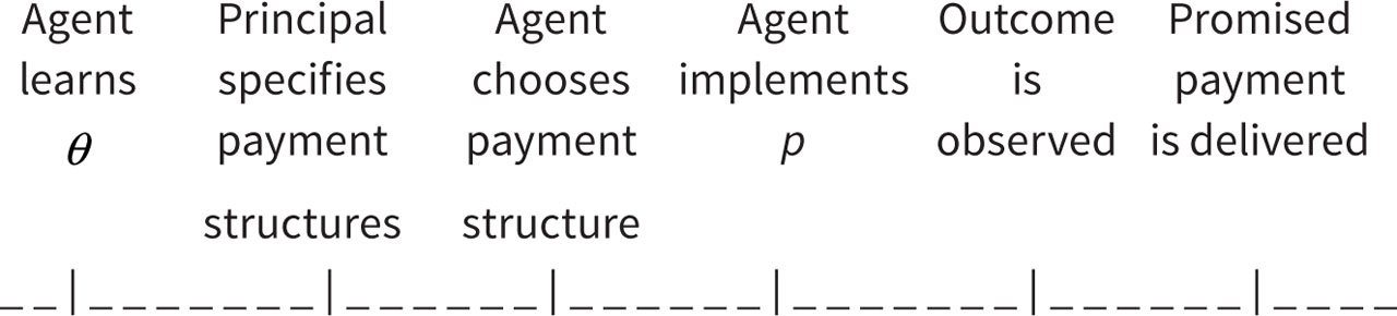This timing is summarized in Figure 1.

Timing in the Setting with Exogenous Ability.

The same timing prevails in the presence of a single payment structure policy (SPP), i.e., when the principal can only offer a single payment structure to the agent. However, the second and third steps in the timing are trivial when an SPP prevails. The principal specifies a single payment structure and the agent simply decides whether to accept the single payment structure or terminate his relationship with the principal. Consequently, in the presence of an SPP, the principal's problem, [PS], is problem [P] with the additional restrictions:

(6)

{\bar{w}}_{H} = {\bar{w}}_{L} and ​ {\underline{w}}_{H} = {\underline{w}}_{L} .

The Full Information Setting

3

As a benchmark, consider the payment structure the principal would implement in the full information setting, where she shares the agent's knowledge of his ability (θ_i) from the outset of their interaction.

Lemma 1

Suppose the agent's ability is θ_i. Then in the full information setting, the principal sets $({\underline{w}}_{i}, {\bar{w}}_{i})$ to ensure ${\bar{w}}_{i} - {\underline{w}}_{i} = \bar{x} - \underline{x}$ and U (θ_i, θ_i) = 0.

In the full information setting, the principal awards the agent the full incremental value of success, i.e., she sets ${\bar{w}}_{i} - {\underline{w}}_{i} = \bar{x} - \underline{x}$ . Doing so induces the agent to implement the success probability that maximizes expected total surplus, i.e., $p_{i}^{s} \equiv \underset{p \in 0, 1]}{arg max} p \bar{x} + 1 - p] \underline{x} - C (p, θ_{i})\}$ . The principal also maximizes her expected profit by setting the payments to eliminate the agent's rent.

Findings in the Setting with Exogenous Ability

4

Now consider the setting of primary interest where the agent is privately informed about his ability from the outset of his interaction with the principal. The payment structures the principal implements in this setting in the absence of an SPP are characterized in Lemma 2. The lemma refers to: (i) $Δ_{x} \equiv \bar{x} - \underline{x}$ , the incremental payoff from project success; and (ii) $Δ_{j} \equiv {\bar{w}}_{j} - {\underline{w}}_{j} for i \in {1, 2}$ , the agent's incremental reward for success when he reports his ability to be θ_j. Throughout the ensuing analysis, we will refer to the agent as “the high-ability agent” when his ability is θ_H, and as the “low-ability agent” when his ability is θ_L.

Lemma 2

At the solution to [P]: (i) Δ_L < Δ_x; (ii) Δ_H = Δ_x; (iii) U (θ_L,θ_L) = 0; and (iv) U (θ_H,θ_H) = U (θ_L,θ_H) > 0.

Lemma 2 reflects standard considerations. 9 The principal eliminates the rent of the low-ability agent. In contrast, the high-ability agent secures rent. This rent is U (θ_L,θ_H), the expected utility the high-ability agent could earn under the $({\underline{w}}_{L}, {\bar{w}}_{L})$ payment structure. To limit this rent, the principal reduces Δ_L below Δ_x and increases ${\underline{w}}_{L}$ sufficiently to ensure U (θ_L,θ_L)= 0. These changes reduce U (θ_L,θ_H) because the high-ability agent implements a higher success probability than the low-ability agent. Therefore, the reduction in Δ_L reduces the agent's expected utility more when he has high ability than when he has low ability. By reducing U (θ_L,θ_H), the principal reduces the rent she must deliver to the high-ability agent to ensure he chooses the $({\underline{w}}_{H}, {\bar{w}}_{H})$ payment structure rather than the $({\underline{w}}_{L}, {\bar{w}}_{L})$ payment structure. Reducing Δ_L thereby enables the principal to reduce ${\underline{w}}_{H}$ while setting Δ_H = Δ_x to ensure the high-ability agent acts to maximize expected total surplus.

In the presence of an SPP, the principal can only implement a single payment structure, $(\underline{w}, \bar{w})$ , where $\underline{w}$ (respectively, $\bar{w}$ ) is the payment the agent receives when the project fails (respectively, succeeds). An SPP thereby makes it more costly for the principal to reduce the incremental reward for success, $Δ \equiv \bar{w} - \underline{w}$ , below Δ_x in order to reduce the rent of the high-ability agent. The reduction in Δ reduces expected total surplus below its maximum possible level both when the agent has low ability and when he has high ability. Consequently, in the presence of an SPP, the principal increases Δ above Δ_L (the incremental reward for success the low-ability agent selects in the absence of an SPP). The principal sets $\underline{w}$ to ensure U (θ_L), the expected utility of the low-ability agent, is zero. 10 This payment structure generates positive expected utility for the high-ability agent (i.e., U (θ_H) > 0), as Lemma 3 reports.

Lemma 3

At the solution to [PS]: (i) Δ ∈(Δ_L, Δ_x); (ii) U (θ_L)= 0; and (iii) U (θ_H) > 0.

Lemmas 2 and 3 underlie the conclusions in Proposition 1. The proposition reports that in the setting with exogenous ability, the presence of an SPP: (i) does not alter the expected utility of the low-ability agent; (ii) increases the expected utility of the high-ability agent; and (iii) reduces the principal's expected profit. The proposition refers to E{Π}, the maximum expected profit the principal can secure in the absence of an SPP, and to E{Π_s}, the principal's corresponding maximum expected profit in the presence of an SPP. 11

Proposition 1

In the setting with exogenous ability: (i) U (θ_L)= U (θ_L, θ_L)= 0, so the low-ability agent never secures rent; (ii) U (θ_H) > U (θ_H,θ_H) > 0, so the high-ability agent always secures rent, and this rent is greater in the presence of an SPP than in its absence; and (iii) E{Π_S} < E{Π}, so an SPP reduces the principal's expected profit.

An SPP increases the expected utility of the high-ability agent in the setting with exogenous ability because Δ > Δ_L. The larger incremental reward for success that the principal implements in the presence of an SPP generates greater rent for the high-ability agent. An SPP reduces the principal's expected profit by restricting her ability to limit the rent of the high-ability agent. This restricted ability compels the principal to deliver more rent to the high-ability agent and induces the principal to reduce expected total surplus below its maximum feasible level when the agent has high ability.

An SPP can either increase or reduce expected welfare. Proposition 2 identifies conditions under which an SPP increases expected welfare by increasing the agent s expected utility more than it reduces the principal's expected profit.

Proposition 2

E{W_S} > E{W}, so an SPP increases expected welfare in the setting with exogenous ability, if $\frac{θ_{H}}{θ_{L}} 1 - ϕ_{H} (\frac{θ_{H}}{θ_{L}} - 1)] > \frac{2 ϕ_{H} - 1}{ϕ_{H}}$ . This inequality holds if ϕ_H is sufficiently close to 0 and $\frac{θ_{H}}{θ_{L}}$ is sufficiently close to 1.

To understand the qualitative conclusions in Proposition 2, recall that an SPP increases expected welfare when the agent has low ability and reduces expected welfare when the agent has high ability (because Δ_H = Δ_x from Lemma 2 and Δ ∈(Δ_L, Δ_x) from Lemma 3). Therefore, an SPP increases expected welfare when θ_L is relatively likely, i.e., when ϕ_H is sufficiently small.

Also, when $\frac{θ_{H}}{θ_{L}}$ is sufficiently large, the principal often sets Δ_L well below Δ_x in the absence of an SPP to limit the agent's rent. An SPP can induce the principal to increase Δ considerably above Δ_L in this case to avoid an excessive reduction in total expected surplus when the agent has high ability. The corresponding increase in expected total surplus when the agent has low ability increases expected welfare.

The Setting with Endogenous Ability

5

The analysis to this point has taken the agent's ability (θ) to be exogenous. We now consider the possibility that the agent might exert personally costly effort to increase the likelihood that his (unobserved) ability is high (θ_H). This effort might entail working diligently to develop or hone skills that enhance the agent's expected performance in working for the principal, for example.

Formally, in the present setting with endogenous ability, the agent can undertake a costly investment in human capital before he interacts with the principal. The more the agent invests in his human capital, the greater is ϕ_H, the probability that he ultimately will be a high-ability agent. We will denote by K (ϕ_H) ≥ 0 the personal cost the agent must incur to ensure he ultimately becomes a high-ability agent with probability ϕ_H. K (·) is a strictly increasing, strictly convex function of ϕ_H. We assume K (·) is such that the agent always implements ϕ_H > 0. 12

The principal observes the agent's expected ability (by observing ϕ_H) before she designs the payment structure(s) for the agent. However, the principal does not observe the agent's actual ability, which the agent learns (privately) before the principal specifies the reward structure(s) under which the agent can operate. Consequently, the information structure in the present setting with endogenous ability parallels the structure in the setting with exogenous ability. The key difference in the present setting is that ϕ_H, and thus the agent's expected ability, is endogenous.

The timing of the interaction between the principal and the agent in the setting with endogenous ability is summarized in Figure 2.

Timing in the Setting with Endogenous Ability.

Although the principal observes the realized value of ϕ_H in the setting with endogenous ability, this value is not contractible. 13 Consequently, the principal cannot explicitly link the agent's payment to the prevailing value of ϕ_H. Such linkage can be difficult in practice when, for example, an accurate assessment of the agent's expected ability requires specialized expertise that only the principal and the agent possess. 14

Although the principal cannot link payments to ϕ_H in the present setting, she can link payments to the realized project performance and to the agent's reported ability, just as in the setting with exogenous ability. Let Ũ(θ_i ;ϕ_H) (respectively, Ũ_S (θ_i ;ϕ_H)) denote the agent's expected utility at the solution to [P] (respectively, [PS]) when his realized ability is θ_i (i ∈{L, H}) and when ϕ_H is the ex ante probability that he will ultimately be a high-ability agent. Then in the setting with endogenous ability, in the absence of an SPP, the agent implements: 15

ϕ_{H}^{*} = \underset{ϕ_{H}}{argmax} ϕ_{H} \tilde{U} (θ_{H}, ϕ_{H}) + 1 - ϕ_{H}] \tilde{U} (θ_{L}; ϕ_{H}) - K (ϕ_{H})\} .

In the presence of an SPP in this setting, the agent implements:

ϕ_{HS}^{*} = \underset{ϕ_{H}}{argmax} ϕ_{H} {\tilde{U}}_{S} (θ_{H}, ϕ_{H}) + 1 - ϕ_{H}] {\tilde{U}}_{S} (θ_{L}; ϕ_{H}) - K (ϕ_{H})\} .

When the agent's ability is endogenous, an SPP can motivate the agent to increase his expected ability (by choosing a higher value for ϕ_H, the probability that he will ultimately be a high-ability agent). This is the case because an SPP induces the principal to implement a payment structure that increases the difference between the equilibrium expected utility of the high-ability agent and the low-ability agent. (Recall Proposition 1.) This increased incremental reward for securing high ability induces the agent to increase his expected ability, as Lemma 4 reports.

Lemma 4

$ϕ_{HS}^{*} > ϕ_{H}^{*}$ .

An SPP also increases the agent's expected utility in the setting with endogenous ability. It does so by limiting the principal's ability to extract the rent of the high-ability agent. This conclusion is recorded formally in Lemma 5. The lemma refers to EU (ϕ_H), the agent's ex ante expected utility in the setting with endogenous ability in the absence of an SPP when the agent implements probability ϕ_H. The lemma also refers to EU_S (ϕ_H), the agent's corresponding expected utility in the presence of an SPP. Formally:

\begin{array}{l} EU (ϕ_{H}) \equiv ϕ_{H} \tilde{U} (θ_{H}; ϕ_{H}) + 1 - ϕ_{H}] \tilde{U} (θ_{L}; ϕ_{H}) - K (ϕ_{H}) and \\ E U_{S} (ϕ_{H}) \equiv ϕ_{H} {\tilde{U}}_{S} (θ_{H}; ϕ_{H}) + 1 - ϕ_{H}] {\tilde{U}}_{S} (θ_{L}; ϕ_{H}) - K (ϕ_{H}) . \end{array}

Lemma 5

$E U_{S} (ϕ_{HS}^{*}) > EU (ϕ_{H}^{*})$ .

The impact of an SPP on the principal's expected profit is less apparent because an SPP introduces two countervailing effects. First, an SPP constrains the principal's ability to extract the agent's rent, which serves to reduce the principal's expected profit. Second, an SPP effectively enables the principal to commit to deliver additional rent to the high-ability agent. The prospect of greater rent induces the agent to increase his expected ability, thereby increasing the expected efficient surplus. 16 This greater surplus serves to increase the principal's expected profit, ceteris paribus. Lemma 6 identifies conditions under which the second effect dominates the first, so an SPP increases the principal's expected profit. The lemma refers to $E Π (ϕ_{H}^{*})$ (respectively, $E Π_{S} (ϕ_{HS}^{*})$ ), the principal's maximum ex ante expected profit in the setting with endogenous ability in the absence of an SPP (respectively, in the presence of an SPP). 17

Lemma 6

$E Π_{S} (ϕ_{HS}^{*}) > E Π (ϕ_{H}^{*}) if \frac{θ_{H}}{θ_{L}}$ is sufficiently large.

For emphasis, the Pareto gains identified in Lemmas 5 and 6 are summarized in Proposition 3.

Proposition 3

$E U_{S} (ϕ_{HS}^{*}) > EU (ϕ_{H}^{*})$ and $E Π_{S} (ϕ_{HS}^{*}) > E Π (ϕ_{H}^{*})$ , so an SPP increases both the agent's expected utility and the principal's expected profit in the setting with endogenous ability, $if \frac{θ_{H}}{θ_{L}}$ is sufficiently large.

Proposition 3 can be viewed an illustration of the principle of the second-best (Lipsey and Lancaster, 1956): in the presence of one friction (the noncontractibility of ϕ_H), an additional friction (an SPP) can sometimes enhance aggregate expected welfare. In addition to increasing expected welfare in the present setting, an SPP can sometimes generate Pareto gains by increasing both the agent's expected utility and the principal's expected profit.

If the principal could explicitly link the agent's payment to his expected ability (ϕ_H), she would not gain by restricting herself to an SPP. This restriction would limit her ability to control the rent of the high-ability agent without enhancing her ability to secure her preferred level of ϕ_H. 18 Consequently, it is the noncontractibility of ϕ_H that renders a commitment to an SPP of potential value to the principal when the agent s ability is endogenous.

Lemma 6 and Proposition 3 indicate that an SPP increases the principal's expected profit and therefore generates Pareto gains when the potential variation in the agent's ability is sufficiently pronounced. As $\frac{θ_{H}}{θ_{L}}$ increases, the rent the high-ability agent can secure under an SPP increases. The prospect of securing greater rent when he has high ability induces the agent to increase ϕ_H. The corresponding increase in the expected efficient surplus enhances the potential for the principal to secure increased expected profit under an SPP, despite her more restricted ability to limit the agent's rent.

It remains to better understand the meaning of the term “sufficiently large” in Proposition 3. It can be shown that Pareto gains arise if $\frac{θ_{H}}{θ_{L}} \geq max 2.8, \frac{10.212 K^{'} (0.5)}{θ_{L} {\bar{x} - \underline{x}]}^{2}}\}$ . 19 However, this sufficient condition is overly restrictive. To illustrate the more general conclusion that an SPP can generate Pareto gains when $\frac{θ_{H}}{θ_{L}}$ is relatively close to 1 and to illustrate that an SPP often can secure substantial Pareto gains, consider Example 1. In this example, $\underline{x} = 1, \bar{x} = 2$ , and θ_L = 0.25. Furthermore, K (ϕ_H) = 0.05(ϕ_H)² is the agent's private cost of ensuring that ϕ_H is the probability that he ultimately has high ability. Table 1 reports the outcomes that arise in Example 1 for several values of θ_H, both in the presence of an SPP and in its absence. Specifically, the table identifies the values of ϕ_H the agent implements, the associated expected utility of the agent, and the corresponding expected profit of the principal. 20

Table 1

The Effects of an SPP in Example 1.

θ_H	$\frac{θ_{H}}{θ_{L}}$	$ϕ_{H}^{*}$	$ϕ_{HS}^{*}$	$EU (ϕ_{H}^{*})$	${EU}_{S} (ϕ_{HS}^{*})$	$E Π (ϕ_{H}^{*})$	$E Π_{S} (ϕ_{HS}^{*})$
0.30	1.2	0.200	0.213	0.0025	0.0026	1.12524	1.12521
0.35	1.4	0.258	0.328	0.0066	0.0078	1.12658	1.12670
0.40	1.6	0.264	0.392	0.0099	0.0131	1.1285	1.12971
0.45	1.8	0.257	0.438	0.0125	0.0180	1.13055	1.13402
0.50	2.0	0.246	0.478	0.0145	0.0227	1.13258	1.13959
0.55	2.2	0.235	0.517	0.0161	0.0272	1.13453	1.14644
0.60	2.4	0.225	0.557	0.0174	0.0316	1.13638	1.15467
0.65	2.6	0.215	0.599	0.0185	0.0361	1.13813	1.16437
0.70	2.8	0.206	0.644	0.0194	0.0406	1.13978	1.17565
0.75	3.0	0.198	0.692	0.0202	0.0453	1.14134	1.18858
0.80	3.2	0.190	0.743	0.0209	0.0502	1.14281	1.20322

Table 1 reports that for the specified parameter values, an SPP increases the agent's expected utility in Example 1 by between 4% (when θ_H = 0.30) and 140% (when θ_H = 0.80). An SPP reduces the principal's expected profit when θ_H = 0.30, but increases her expected profit when θ_H ≥ 0.35. 21 The gains for the principal range from 0.01% when θ_H = 0.35 to nearly 5.3% when θ_H = 0.80.

The finding that an SPP generates Pareto gains $if \frac{θ_{H}}{θ_{L}} \geq max 2.8, \frac{10.212 K^{'} (0.5)}{θ_{L} {[\bar{x} - \underline{x}]}^{2}}\}$ suggests that $\hat{\frac{θ_{H}}{θ_{L}}}$ , the smallest value of $\frac{θ_{H}}{θ_{L}}$ above which an SPP ensures Pareto gains, may increase as it becomes more costly for the agent to increase ϕ_H. 22 Numerical solutions confirm that this relationship holds under a broad set of conditions. To illustrate, consider Example 2 in which $\underline{x} = 1, \bar{x} = 2$ , θ_L = 0.25, and $K (ϕ_{H}) = \frac{k}{2} {(ϕ_{H})}^{2}$ . Table 2 reports that $\hat{\frac{θ_{H}}{θ_{L}}}$ declines monotonically as k declines in Example 2. The smaller is the agent's cost of increasing ϕ_H, the larger is the value of ϕ_H the agent will implement in the presence of an SPP, ceteris paribus. Consequently, as k declines, the agent will increase ϕ_H to the level that ensures Pareto gains even when $\frac{θ_{H}}{θ_{L}}$ is smaller.

Table 2

The Minimum $\frac{θ_{H}}{θ_{L}}$ that Ensures Pareto Gains in Example 2.

k	$\hat{\frac{θ_{H}}{θ_{L}}}$	k	$\hat{\frac{θ_{H}}{θ_{L}}}$	k	$\hat{\frac{θ_{H}}{θ_{L}}}$
0.10	1.34	0.25	1.56	1.0	2.18
0.15	1.44	0.50	1.88	2.0	2.72
0.20	1.52	0.75	2.00	5.0	3.68

Conclusions

6

We have examined the effects of a single payment structure policy (SPP) in the presence of moral hazard and adverse selection. We have shown that the effects of an SPP can vary according to whether the agent's ability is exogenous or endogenous. When the agent's ability is exogenous, an SPP reduces the principal's expected profit and increases the agent's expected utility. It does so by restricting the principal's ability to limit the rent of the high-ability agent. When the agent's ability is endogenous, an SPP can increase both the principal's expected profit and the agent's expected utility. This is the case because by restricting the principal's ability to limit the rent of the high-ability agent, an SPP induces the agent to increase ϕ_H, the probability that the agent ultimately has high ability. The corresponding increase in the expected efficient surplus admits the possibility of Pareto gains. Such gains can be particularly likely to arise when the potential variation in the agent's ability is relatively pronounced, when it is not very costly for the agent to increase ϕ_H, and when the principal lacks alternative means to credibly promise to reward the agent for enhancing his (noncontractible) human capital (i.e., for increasing his expected ability in performing the principal's idiosyncratic task).

Our analysis suggests that a common view of optional compensation structures may merit more nuanced consideration in some settings. The common view is that employers often can gain by encouraging employees to choose among simple, carefully-designed compensation structures (e.g., Bommaraju and Hohenberg, 2018, p. 122). This conclusion is certainly correct when employee ability is largely exogenous. The conclusion also can be correct when employee ability is endogenous. However, as we have shown, the conclusion is not always correct in this case. Consequently, when designing compensation structures, employers should consider not only the optimal design of optional compensation structures, but also whether it might be preferable to preclude any choice among compensation schedules in order to motivate employees to undertake ability-enhancing investment in human capital.

We have shown that an SPP can generate Pareto gains when it induces the agent to increase ϕ_H, the probability that the agent ultimately has high ability. An SPP would not secure Pareto gains if the principal, rather than the agent, were the party that could devote personally costly effort to increase ϕ_H. In such a setting, an SPP compels the principal to deliver more rent to the high-ability agent, thereby reducing the principal's incentive to increase ϕ_H.

We have focused on the interaction between an employer and a worker, for concreteness. However, our analysis is relevant more broadly. For example, our conclusions also hold in a setting where a regulator attempts to motivate a regulated firm to improve its performance (e.g., reduce its operating costs or improve it service quality). When the regulator cannot reward the firm directly for enhancing its expected ability to improve its performance (because the expected ability is not contractible), the regulator can motivate the firm to undertake ability-enhancing effort by adopting an SPP. 23

We have considered a binary adverse selection problem for analytic tractability. However, the same forces we have identified will prevail more generally. An SPP will continue to reduce the principal's expected profit when the agent's expected ability is exogenous. In contrast, by enhancing the agent's rent for the higher ability realizations, an SPP can encourage the agent to increase the likelihood of the highest possible ability realizations. The corresponding enhanced expected efficient surplus introduces the potential for Pareto gains from an SPP.

In addition to considering non-binary adverse selection settings, future research might explore competition among principals. 24 Such competition may limit the conditions under which an SPP will generate Pareto gains. When principals compete for an agent's services, the agent generally will secure a relatively large fraction of the increased expected efficient surplus that arises when an SPP induces the agent to increase his expected ability. Consequently, even when an SPP serves to increase the expected efficient surplus, little of the incremental potential surplus may flow to principals.

†

We thank the editor, Pierre Cahuc, three anonymous referees, and Ramarao Desiraju for very helpful comments and suggestions.

Appendices

Appendix

Part A of this Appendix records the payments the principal will implement in the setting of Example 1 for selected values of θ_H. Part B presents the proofs of the formal conclusions in the text.

Optimal Payments in the Setting of Example 1

A

Table A1

Optimal Payments in the Setting of Example 1.

	θ_H = 0.3	θ_H = 0.4	θ_H = 0.5	θ_H = 0.6	θ_H = 0.7	θ_H = 0.8
${\underline{W}}_{L}$	− 0.113	− 0.085	− 0.071	− 0.063	− 0.058	− 0.054
${\bar{W}}_{L}$	0.839	0.738	0.683	0.648	0.623	0.605
Δ_L	0.952	0.823	0.754	0.711	0.681	0.659
${\underline{W}}_{H}$	− 0.127	− 0.149	− 0.179	− 0.212	− 0.246	− 0.280
${\bar{W}}_{H}$	0.873	0.851	0.821	0.788	0.754	0.720
Δ_H	1.0	1.0	1.0	1.0	1.0	1.0
$\underline{W}$	− 0.115	− 0.088	− 0.071	− 0.060	− 0.053	− 0.048
$\bar{W}$	0.845	0.752	0.684	0.635	0.598	0.570
Δ	0.961	0.840	0.756	0.695	0.651	0.617

Proofs of Formal Conclusions in the Text

B

Proof of Lemma 2

We will demonstrate that the solution to the following relaxed problem, [P]^′, is a feasible solution to [P], and therefore is a solution to [P].

The Principal's Relaxed Problem, [P]′

(7)

\begin{array}{l} \underset{{\underline{w}}_{L}, {\bar{w}}_{L}, {\underline{w}}_{H}, {\bar{w}}_{H}}{Maximize} ϕ_{L} [p_{L} (\bar{x} - {\bar{w}}_{L}) + (1 - p_{L}) (\underline{x} - {\underline{w}}_{L})] \\ + ϕ_{H} [p_{H} (\bar{x} - {\bar{w}}_{H}) + (1 - p_{H}) (\underline{x} - {\underline{w}}_{H})] \end{array}

subject to:

(8)

p_{L} {\bar{w}}_{L} + [1 - p_{L}] {\underline{w}}_{L} - C (p_{L}, θ_{L}) \geq 0; and

(9)

p_{H} {\bar{w}}_{H} + [1 - p_{H}] {\underline{w}}_{H} - C (p_{H}, θ_{H}) \geq max_{p} {p {\bar{w}}_{L} + [1 - p] {\underline{w}}_{L} - C (p, θ_{H})} .

Characterizing the Solution to [P]′

For i ∈ {L, H}, p_i is defined by: 25

(10)

C_{p} (p_{i}, θ_{i}) = {\bar{w}}_{i} = {\underline{w}}_{i} \Rightarrow \frac{\partial p_{i}}{\partial {\underline{w}}_{i}} = - \frac{1}{c_{pp} (p_{i}, θ_{i})} < 0 and \frac{\partial p_{i}}{\partial {\bar{w}}_{i}} = \frac{1}{c_{pp} (p_{i}, θ_{i})} > 0 .

For i, j ∈ {L, H}(j ≠ i), let ${\hat{p}}_{i}$ be defined by:

(11)

C_{p} ({\hat{p}}_{i}, θ_{i}) = {\bar{w}}_{j} - {\underline{w}}_{j} \Rightarrow \frac{\partial {\hat{p}}_{i}}{\partial {\underline{w}}_{j}} = - \frac{1}{c_{pp} ({\hat{p}}_{i}, θ_{i})} < 0 and \frac{\partial {\hat{p}}_{i}}{\partial {\bar{w}}_{j}} = \frac{1}{c_{pp} ({\hat{p}}_{i}, θ_{i})} > 0 .

Let λ_L ≥ 0 and μ_H ≥ 0 denote the Lagrange multipliers associated with (8) and (9), respectively. The Lagrangian for [P]^′ is:

(12)

\begin{array}{l} ℒ = ϕ_{L} [p_{L} (\bar{x} - {\bar{w}}_{L}) + (1 - p_{L}) (\underline{x} - {\underline{w}}_{L})] + ϕ_{H} [p_{H} (\bar{x} - {\bar{w}}_{H}) + (1 - p_{H}) (\underline{x} - {\underline{w}}_{H})] \\ + λ_{L} [p_{L} {\bar{w}}_{L} + (1 - p_{L}) {\underline{w}}_{L} - C (p_{L}, θ_{L})] \\ + μ_{H} [p_{H} {\bar{w}}_{H} + (1 - p_{H}) {\underline{w}}_{H} - C (p_{H}, θ_{H}) \\ - {\hat{p}}_{H} {\bar{w}}_{L} - (1 - {\hat{p}}_{H}) {\underline{w}}_{L} + C ({\hat{p}}_{H}, θ_{H})] . \end{array}

(10) – (12) imply that the necessary conditions for a solution to [P]^′ include:

(13)

\begin{array}{l} \frac{\partial ℒ}{\partial {\bar{w}}_{L}} = ϕ_{L} [- p_{L} + (\bar{x} - {\bar{w}}_{L}) \frac{\partial p_{L}}{\partial {\bar{w}}_{L}} - (\underline{x} - {\underline{w}}_{L}) \frac{\partial p_{L}}{\partial {\bar{w}}_{L}}] \\ + λ_{L} [p_{L} + {\bar{w}}_{L} \frac{\partial p_{L}}{\partial {\bar{w}}_{L}} - {\underline{w}}_{L} \frac{\partial p_{L}}{\partial {\bar{w}}_{L}} - C_{p} (p_{L}, θ_{L}) \frac{\partial p_{L}}{\partial {\bar{w}}_{L}}] \\ - μ_{H} [{\hat{p}}_{H} + {\bar{w}}_{L} \frac{\partial {\hat{p}}_{H}}{\partial {\bar{w}}_{L}} - {\underline{w}}_{L} \frac{\partial {\hat{p}}_{H}}{\partial {\bar{w}}_{L}} - C_{p} ({\hat{p}}_{H}, θ_{H}) \frac{\partial {\hat{p}}_{H}}{\partial {\bar{w}}_{L}}] \\ = ϕ_{L} [- p_{L} + \frac{\bar{x} - {\bar{w}}_{L} - (\underline{x} - {\underline{w}}_{L})}{C_{pp} (p_{L}, θ_{L})}] + λ_{L} [p_{L} + \frac{{\bar{w}}_{L} - {\underline{w}}_{L} - C_{p} (p_{L}, θ_{L})}{C_{pp} (p_{L}, θ_{L})}] \\ - μ_{H} [{\hat{p}}_{H} + \frac{{\bar{w}}_{L} - {\underline{w}}_{L} - C_{p} ({\hat{p}}_{H}, θ_{H})}{C_{pp} (p_{L}, θ_{H})}] = 0 . \end{array}

(14)

\begin{array}{l} \frac{\partial ℒ}{\partial {\underline{w}}_{L}} = - ϕ_{L} [1 - p_{L} + \frac{\bar{x} - {\bar{w}}_{L} - (\underline{x} - {\underline{w}}_{L})}{C_{pp} (p_{L}, θ_{L})}] + λ_{L} [1 - p_{L} - \frac{{\bar{w}}_{L} - {\underline{w}}_{L} - C_{p} (p_{L}, θ_{L})}{C_{pp} (p_{L}, θ_{L})}] \\ - μ_{H} [1 - {\hat{p}}_{H} - \frac{{\bar{w}}_{L} - {\underline{w}}_{L} - C_{p} ({\hat{p}}_{H}, θ_{H})}{C_{pp} ({\hat{p}}_{H}, θ_{H})}] = 0 . \end{array}

(15)

\begin{array}{l} \frac{\partial ℒ}{\partial {\bar{w}}_{H}} = ϕ_{H} [- p_{H} + \frac{\bar{x} - {\bar{w}}_{H} - (\underline{x} - {\underline{w}}_{H})}{C_{pp} (p_{H}, θ_{H})}] \\ + μ_{H} [p_{H} + \frac{{\bar{w}}_{H} - {\underline{w}}_{H} - C_{p} (p_{H}, θ_{H})}{C_{pp} (p_{H}, θ_{H})}] = 0 . \end{array}

(16)

\begin{array}{l} \frac{\partial ℒ}{\partial {\underline{w}}_{H}} = - ϕ_{H} [1 - p_{H} + \frac{\bar{x} - {\bar{w}}_{H} - (\underline{x} - {\underline{w}}_{H})}{C_{pp} (p_{H}, θ_{H})}] \\ + μ_{H} [1 - p_{H} - \frac{{\bar{w}}_{H} - {\underline{w}}_{H} - C_{p} (p_{H}, θ_{H})}{C_{pp} (p_{H}, θ_{H})}] = 0 . \end{array}

Adding (13) and (14) provides:

(17)

- ϕ_{L} + λ_{L} - μ_{H} = 0 .

Adding (15) and (16) provides:

(18)

\begin{array}{l} - ϕ_{H} + μ_{H} = 0 \Rightarrow μ_{H} = ϕ_{H} > 0 \\ \Rightarrow U (θ_{H}, θ_{H}) \equiv p_{H} {\bar{w}}_{H} + [1 - p_{H}] {\underline{w}}_{H} - C (p_{H}, θ_{H}) \\ = {\hat{p}}_{H} {\bar{w}}_{L} + [1 - {\hat{p}}_{H}] {\underline{w}}_{L} - C ({\hat{p}}_{H}, θ_{H}) \equiv U (θ_{L}, θ_{H}) . \end{array}

(17) and (18) imply λ_L = ϕ_L + ϕ_H = 1>0

(19)

\Rightarrow U (θ_{L}, θ_{L}) \equiv p_{L} {\bar{w}}_{L} + [1 - p_{L}] {\underline{w}}_{L} - C (p_{L}, θ_{L}) = 0 .

Because μ_H = ϕ_H, (15) implies:

(20)

\begin{array}{l} \bar{x} - {\bar{w}}_{H} - (\underline{x} - {\underline{w}}_{H}) + {\bar{w}}_{H} - {\underline{w}}_{H} - C_{P} (p_{H}, θ_{H}) = 0 \\ \Rightarrow C_{p} (p_{H}, θ_{H}) = \bar{x} - \underline{x} \Rightarrow Δ_{H} \equiv {\bar{w}}_{H} - {\underline{w}}_{H} = \bar{x} - \underline{x} \equiv Δ_{x} . \end{array}

(10), (11), (13), (18), and (19) imply:

(21)

\begin{array}{l} ϕ_{L} [- p_{L} + \frac{\bar{x} - {\bar{w}}_{L} - (\underline{x} - {\underline{w}}_{L})}{C_{pp} (p_{L}, θ_{L})}] + p_{L} - ϕ_{L} {\hat{p}}_{H} = 0 \\ \Rightarrow ϕ_{L} [\frac{\bar{x} - {\bar{w}}_{L} - (\underline{x} - {\underline{w}}_{L})}{C_{pp} (p_{L}, θ_{L})}] = ϕ_{H} [{\hat{p}}_{H} - p_{L}] \\ \Rightarrow \bar{x} - \underline{x} - ({\bar{w}}_{L} - {\underline{w}}_{L}) = C_{pp} (p_{L}, θ_{L}) \frac{ϕ_{H}}{ϕ_{L}} [{\hat{p}}_{H} - p_{L}] . \end{array}

(10) and (11) imply that when the agent with the ability θ choose the $({\underline{w}}_{L}, {\bar{w}}_{L})$ payment structure, his choice of p is determined by:

(22)

\begin{array}{l} C_{p} (p, θ) = {\bar{w}}_{L} - {\underline{w}}_{L} \Rightarrow C_{pp} (p, θ) dp + C_{p θ} (p, θ) d θ = 0 \\ \Rightarrow \frac{dp}{d θ} = - \frac{C_{p θ} (p, θ)}{C_{pp} (p, θ)} > 0 \Rightarrow {\hat{p}}_{H} > p_{L} . \end{array}

(21) and (22) imply:

(23)

Δ_{L} \equiv {\bar{w}}_{L} - {\underline{w}}_{L} < \bar{x} - \underline{x} \equiv Δ_{x} .

Verifying that the solution to [P]′ is a Feasible Solution to [P]

It remains to verify that (4) holds when i = H and that (5) holds when i = L. The following Finding is helpful in this regard. The Finding refers to $\tilde{U} (Δ_{i}, θ) \equiv \underset{p \in [0, 1]}{maximum} {{\underline{w}}_{i} + p Δ_{i} - C (p, θ)}$ , where $Δ_{i} \equiv {\bar{w}}_{i} - {\underline{w}}_{i}$ .

Finding 1

$\tilde{U} (Δ_{i}, θ) - \tilde{U} ({\hat{Δ}}_{i}, θ)$ is non-decreasing in θ for all $Δ_{i} > {\hat{Δ}}_{i} \geq 0$ .

Proof

Observe that for $Δ_{i} > {\hat{Δ}}_{i} \geq 0$ :

(24)

\begin{array}{l} \frac{d [\tilde{U} (Δ_{i}, θ) - \tilde{U} ({\hat{Δ}}_{i}, θ)]}{d θ} = \frac{d {\tilde{p}}_{i}}{d θ} [Δ_{i} - C_{p} ({\tilde{p}}_{i}, θ) - C_{θ} ({\tilde{p}}_{i}, θ)] - \frac{d {\hat{p}}_{i}}{d θ} [\hat{Δ} - C_{p} ({\hat{p}}_{i}, θ)] + C_{θ} ({\hat{p}}_{i}, θ) \\ = C_{θ} ({\hat{p}}_{i}, θ) - C_{θ} ({\tilde{p}}_{i}, θ) \geq 0 \end{array}

where

Δ_{i} = C_{p} ({\tilde{p}}_{i}, θ)

and

{\hat{Δ}}_{i} = C_{p} ({\hat{p}}_{i}, θ)

. The last inequality in (24) holds because

{\tilde{p}}_{i} > {\hat{p}}_{i}

(since

Δ_{i} > {\hat{Δ}}_{i}

) and C_p (p, θ_H) < C_p (p, θ_L for all p ∈ (1, 0).

To verify that (4) holds when i = H, observe that:

(25)

\begin{array}{l} U (θ_{H}, θ_{H}) \equiv p_{H} {\bar{w}}_{H} + [1 - p_{H}] {\underline{w}}_{H} - C (p_{H}, θ_{H}) = {\hat{p}}_{H} {\bar{w}}_{L} + [1 - {\hat{p}}_{H}] {\underline{w}}_{L} - C ({\hat{p}}_{H}, θ_{H}) \\ \geq p_{L} {\bar{w}}_{L} + [1 - p_{L}] {\underline{w}}_{L} - C (p_{L}, θ_{H}) \geq p_{L} {\bar{w}}_{L} [1 - p_{L}] {\underline{w}}_{L} - C (p_{L}, θ_{L}) \\ \geq p_{L} {\bar{w}}_{L} + [1 - p_{L}] {\underline{w}}_{L} - C (p_{L}, θ_{L}) \equiv U (θ_{L}, θ_{L}) = 0 . \end{array}

The equality in (25) reflects (18). The first inequality in (25) holds because ${\hat{p}}_{H} = argmax {p {\bar{w}}_{L} - [1 - p] {\underline{w}}_{L} + C (p, θ_{H})}$ . The second inequality in (25) holds because C(p, θ_L) ≥ C(p, θ_H) for all p ≥ 0. The last equality in (25) reflects (19).

To verify that (5) holds when i = L, observe that Δ_H > Δ_L from (20) and (23). Therefore, (18) implies:

(26)

U (θ_{H}, θ_{H}) - U (θ_{L}, θ_{H}) = 0 \Rightarrow U (θ_{H}, θ_{L}) - U (θ_{L}, θ_{L}) \leq 0 .

The inequality in (26) reflects Finding 1. (26) implies that U (θ_L,θ_L) ≥ U (θ_H,θ_L), so (5) holds when i = L at the solution to [P]^′.

Definition.

(27)

p_{i}^{'} = \underset{p}{argmax} {p \bar{w} + [1 - p] \underline{w} - C (p, θ_{i})} for i \in {L, H} .

Proof of Lemma 3

The proof of the Lemma follows from Findings 2 – 7.

Finding 2

At the solution to [PS]:

(28)

p_{H}^{'} \bar{w} + [1 - p_{H}^{'}] \underline{w} - C (p_{H}^{'}, θ_{H}) > p_{L}^{'} \bar{w} + [1 - p_{L}^{'}] \underline{w} - C (p_{L}^{'}, θ_{L}) .

Proof

Observe that:

(29)

\begin{array}{l} p_{H}^{'} \bar{w} + [1 - p_{H}^{'}] \underline{w} - C (p_{H}^{'}, θ) = p_{L}^{'} \bar{w} + [1 - p_{L}^{'}] \underline{w} - C (p_{L}^{'}, θ_{L}) \\ + [\bar{w} - \underline{w}] [p_{H}^{'} - p_{L}^{'}] - [C (p_{H}^{'}, θ_{H}) - C (p_{L}^{'}, θ_{L})] . \end{array}

(27) implies that $p_{H}^{'} > p_{L}^{'}$ because C_p (p,θ_H) < C_p (p,θ_L) for all p > 0. Furthermore:

(30)

\begin{array}{l} [\bar{w} - \underline{w}] [p_{H}^{'} - p_{L}^{'}] = \int_{p_{L}^{'}}^{p_{H}^{'}} [\bar{w} - \underline{w}] dp > \int_{p_{L}^{'}}^{p_{H}^{'}} C_{p} (p, θ_{H}) dp \\ = C (p_{H}^{'}, θ_{H}) - C (p_{L}^{'}, θ_{H}) > C (p_{H}^{'}, θ_{H}) - C (p_{L}^{'}, θ_{L}) . \end{array}

The first inequality in (30) holds because for all $p < p_{H}^{'}$ :

(31)

C_{p} (p, θ_{H}) < C_{p} (p_{H}^{'}, θ_{H}) = \bar{w} - \underline{w} .

The inequality in (31) holds because C(·) is a strictly convex function of P. The equality (31) reflects (27). (29) and (30) imply that (28) holds.

Finding 3

At the solution to [PS]:

(32)

U (θ_{L}) \equiv p_{L}^{'} \bar{w} + [1 - p_{L}^{'}] \underline{w} - C (p_{L}^{'}, θ_{L}) = 0 and

(33)

U (θ_{H}) \equiv p_{H}^{'} \bar{w} + [1 - p_{H}^{'}] \underline{w} - C (p_{H}^{'}, θ_{H}) > 0 .

The conclusion follows directly from (4) and Finding 2.

Finding 4

At the solution to [PS]:

Δ \equiv \bar{w} - \underline{w} < \bar{x} - \underline{x} \equiv Δ_{x}, so p_{L}^{'} < p_{L}^{*} and p_{L}^{'} < p_{H}^{*} .

Proof

(27) implies:

(34)

C_{p} (p_{L}^{'}, θ_{L}) = C_{p} (p_{H}^{'}, θ_{H}) = \bar{w} - \underline{w}

(35)

\Rightarrow \frac{\partial p_{i}^{'}}{\partial \underline{w}} = - \frac{1}{c_{pp} (p_{i}, θ_{i})} < 0 and \frac{\partial p_{i}^{'}}{\partial \bar{w}} = \frac{1}{c_{pp} (p_{i}, θ_{i})} > 0 .

Let λ ≥ 0 denote the Langrange multiplier associated with (4) for i = L. Then Finding 3 implies that the Lagrangian for [PS] is:

\begin{array}{l} ℒ^{'} = [ϕ_{L} p_{L}^{'} + ϕ_{H} p_{H}^{'}] [\bar{x} - \bar{x}] + [1 - ϕ_{L} p_{L}^{'} - ϕ_{H} p_{H}^{'}] [\underline{x} - \underline{w}] \\ + λ [p_{L}^{'} \bar{w} + (1 - p_{L}^{'}) \underline{w} - C (p_{L}^{'}, θ_{L}] . \end{array}

One necessary condition for a solution to [PS] is:

(36)

\begin{array}{l} \frac{\partial ℒ^{'}}{\partial \bar{w}} = - [ϕ_{L} p_{L}^{'} + ϕ_{H} p_{H}^{'}] + [\bar{\underline{x}} - \bar{w}] [ϕ_{L} \frac{\partial p_{L}^{'}}{\partial \bar{w}} + ϕ_{H} \frac{\partial p_{H}^{'}}{\partial \bar{w}}] \\ - [\underline{x} - \underline{w}] [ϕ_{L} \frac{\partial p_{L}^{'}}{\partial \bar{w}} + ϕ_{H} \frac{\partial p_{H}^{'}}{\partial \bar{w}}] + λ [p_{L}^{'} + \frac{\partial p_{L}^{'}}{\partial \bar{w}} (\bar{w} - \underline{w} - C_{p} (p_{L}^{'}, θ_{L}))] \\ = [\frac{ϕ_{L}}{C_{pp} (p_{L}^{'}, θ_{L})} + \frac{ϕ_{H}}{C_{pp} (p_{H}^{'}, θ_{H})}] [\bar{x} - \underline{x} - (\bar{w} - \underline{w})] \\ - [ϕ_{L} p_{L}^{'} + ϕ_{H} p_{H}^{'}] + λ p_{L}^{'} = 0 . \end{array}

The last equality in (36) reflects (34) and (35).

An additional necessary condition for a solution to [PS] is:

(37)

\begin{array}{l} \frac{\partial ℒ^{'}}{\partial \underline{w}} = - [1 - ϕ_{L}^{'} p_{L}^{'} + ϕ_{H} p_{H}^{'}] + [\bar{x} - \underline{x} - (\bar{w} - \underline{w})] [ϕ_{L} \frac{\partial p_{L}^{'}}{\partial \underline{w}} + ϕ_{H} \frac{\partial p_{H}^{'}}{\partial \underline{w}}] \\ + λ [1 - p_{L}^{'} + \frac{\partial p_{L}^{'}}{\partial \underline{w}} (\bar{w} - \underline{w} - C_{p} (p_{L}^{'}, θ_{L}))] \\ = - [\frac{ϕ_{L}}{C_{pp} (p_{L}^{'}, θ_{L})} + \frac{ϕ_{H}}{C_{pp} (p_{H}^{'}, θ_{H})}] [\bar{x} - \underline{x} - (\bar{w} - w)] \\ - 1 + ϕ_{L} p_{L}^{'} + ϕ_{H} p_{H}^{'} + λ [1 - p_{L}^{'}] = 0 . \end{array}

Adding (36) and (37) reveals that λ = 1. Therefore, (36) implies:

(38)

\begin{array}{l} [\frac{ϕ_{L}}{C_{pp} (p_{L}^{'}, θ_{L})} + \frac{ϕ_{H}}{C_{pp} (p_{H}^{'}, θ_{H})}] [\bar{x} - \underline{x} - (\bar{w} - \underline{w})] = ϕ_{H} [p_{H}^{'} - p_{L}^{'}] \\ \Rightarrow \bar{x} - \underline{x} - (\bar{w} - \underline{w}) = \frac{ϕ_{H} [p_{H}^{'} - p_{L}^{'}]}{\frac{ϕ_{L}}{C_{pp} (p_{L}^{'}, θ_{L})} + \frac{ϕ_{H}}{C_{pp} (p_{H}^{'}, θ_{H})}} > 0 . \end{array}

The inequality in (38) holds because the agent's choice of P^′ is determined by:

\begin{array}{l} C_{p} (p^{'}, θ) = \bar{w} - \underline{w} \Rightarrow C_{pp} (p^{'}, θ) dp + C_{p θ} (p^{'}, θ) d θ = 0 \\ \Rightarrow \frac{d p^{'}}{d θ} = - \frac{C_{p θ} (p^{'}, θ)}{C_{pp} (p ’ θ)} > 0 \Rightarrow p_{H}^{'} > p_{L}^{'} . \end{array}

Finding 5

U (θ_H) > U (θ_H,θ_H)if Δ > Δ_L.

Proof

Recall from (18) that:

(39)

U (θ_{H}, θ_{H}) = U (θ_{L}, θ_{H}) \equiv {\hat{p}}_{H} {\bar{w}}_{L} + [1 - {\hat{p}}_{H}] {\underline{w}}_{L} - C ({\hat{p}}_{H}, θ_{H}) .

Because $p_{H}^{'} = \underset{p}{argmax} {p \bar{w} + [1 - p] \underline{w} - C (p, θ_{H})}$ :

(40)

p_{H}^{'} \bar{w} + [1 - p_{H}^{'}] \underline{w} - C (p_{H}^{'}, θ_{H}) \geq {\hat{p}}_{H} \bar{w} + [1 - {\hat{p}}_{H}] \underline{w} - C (p_{H}^{'}, θ_{H}) .

(39) and (40) imply that U (θ_H) > U (θ_H,θ_H) if:

(41)

\begin{array}{l} {\hat{p}}_{H} \bar{w} + [1 - {\hat{p}}_{H}] \underline{w} - C ({\hat{p}}_{H}, θ_{H}) > {\hat{p}}_{H} \bar{w_{L}} + [1 - {\hat{p}}_{H}] \underline{w_{L}} - C (p_{H}^{'}, θ_{H}) \\ \Leftrightarrow {\hat{p}}_{H} \bar{w} + [1 - {\hat{p}}_{H}] \underline{w} > {\hat{p}}_{H} {\bar{w}}_{L} + [1 - {\hat{p}}_{H}] {\underline{w}}_{L} . \end{array}

$p_{L}^{'} > p_{L}$ because $\bar{w} - \underline{w} > {\bar{w}}_{L} - {\underline{w}}_{L}$ , by assumption. Furthermore, ${\hat{p}}_{H} > p_{L}$ because C_p (p,θ_H) > C_p (p,θ_L) for all p > 0. Therefore, there are two cases to consider.

Case 1. ${\hat{p}}_{H} \geq p_{L}^{'} > p_{L}$ .

Because U (θ_L)= 0 from (32):

(42)

\begin{array}{l} \underline{w} + [\bar{w} - \underline{w}] p_{L}^{'} = C (p_{L}^{'}, θ_{L}) = C (p_{L}, θ_{L}) + \int_{p_{L}}^{p_{L}^{'}} C_{p} (p, θ_{L}) dp \\ > C (p_{L}, θ_{L}) + \int_{p_{L}}^{p_{L}^{'}} [{\bar{w}}_{L} - {\underline{w}}_{L}] dp = C (p_{L}, θ_{L}) + [{\bar{w}}_{L} - {\underline{w}}_{L}] [p_{L}^{'} - p_{L}] . \end{array}

The inequality in (42) holds because $C (p_{L}, θ_{L}) = {\bar{w}}_{L} - {\underline{w}}_{L}$ and C(·) is strictly a convex function of P.

Because U (θ_L,θ_L)= 0 from (19), ${\underline{w}}_{L} + [{\bar{w}}_{L} - {\underline{w}}_{L}] p_{L} = C (p_{L}, θ_{L})$

(43)

\begin{array}{l} \Rightarrow C (p_{L}, θ_{L}) + [{\bar{w}}_{L} - {\underline{w}}_{L}] [p_{L}^{'} - p_{L}] \\ = {\underline{w}}_{L} + [{\bar{w}}_{L} - {\underline{w}}_{L}] p_{L} + [{\bar{w}}_{L} - {\underline{w}}_{L}] [p_{L}^{'} - p_{L}] = {\underline{w}}_{L} + [{\bar{w}}_{L} - {\underline{w}}_{L}] p_{L}^{'} . \end{array}

(42) and (43) imply:

(44)

\begin{array}{l} \underline{w} + [\bar{w} - \underline{w}] p_{L}^{'} > {\underline{w}}_{L} + [{\bar{w}}_{L} - {\underline{w}}_{L}] p_{L}^{'} \\ \Rightarrow \underline{w} + [\bar{w} - \underline{w} - ({\bar{w}}_{L} - {\underline{w}}_{L})] p_{L}^{'} > {\underline{w}}_{L} \\ \Rightarrow \underline{w} + [\bar{w} - \underline{w} - ({\bar{w}}_{L} - {\underline{w}}_{L})] {\hat{p}}_{H} > {\underline{w}}_{L} \\ \Rightarrow \underline{w} + [\bar{w} - \underline{w}] {\hat{p}}_{H} > {\underline{w}}_{L} + [{\bar{w}}_{L} - {\underline{w}}_{L}] {\hat{p}}_{H} . \end{array}

The third line in (44) hold because $\bar{w} - \underline{w} > {\bar{w}}_{L} - {\underline{w}}_{L}$ (by assumption) and ${\hat{p}}_{H} \geq p_{L}^{'}$ in the present case. (44) implies that (41) holds.

Case II. $p_{L}^{'} > {\hat{p}}_{H} > p_{L}$ .

Because U (θ_L)= 0 from (32), $p_{L}^{'} \bar{w} + [1 - p_{L}^{'}] \underline{w} = C (p_{L}^{'}, θ_{L})$

(45)

\Rightarrow C (p_{L}^{'}, θ_{L}) - C (p_{L}^{'}, θ_{H}) = p_{L}^{'} \bar{w} + [1 - p_{L}^{'}] \underline{w} - C (p_{L}^{'}, θ_{H}) .

Because $p_{H}^{'} = \underset{p}{argmax} {p \bar{w} + [1 - p] \underline{w} - C (p, θ_{H})}$ :

(46)

U (θ_{H}) > p_{L}^{'} \bar{w} + [1 - p_{L}^{'}] \underline{w} - C (p_{L}^{'}, θ_{H}) .

(45) and (46) imply:

(47)

U (θ_{H}) > C (p_{L}^{'}, θ_{L}) - C (p_{L}^{'}, θ_{H}) .

Because U (θ_L,θ_L)= 0 from (19):

(48)

\begin{array}{l} {\underline{w}}_{L} + p_{L} [{\bar{w}}_{L} - {\underline{w}}_{L}] = C (p_{L}, θ_{L}) = C ({\hat{p}}_{H}, θ_{L}) - \int_{p_{L}}^{{\hat{p}}_{H}} C_{p} (p, θ_{L}) dp \\ < C ({\hat{p}}_{H}, θ_{L}) - \int_{p_{L}}^{{\hat{p}}_{H}} [{\bar{w}}_{L} - {\underline{w}}_{L}] dp = C ({\hat{p}}_{H}, θ_{L}) - [{\bar{w}}_{L} - {\underline{w}}_{L}] [{\hat{p}}_{H} - p_{L}] . \end{array}

The inequality in (48) holds because $C (p_{L}, θ_{L}) = {\bar{w}}_{L} - {\underline{w}}_{L}$ and C(·) is a strictly convex function of P. (48) implies:

(49)

{\underline{w}}_{L} < C ({\hat{p}}_{H}, θ_{L}) - {\hat{p}}_{H} [{\bar{w}}_{L} - {\underline{w}}_{L}] \Rightarrow {\hat{p}}_{H} {\bar{w}}_{L} + [1 - {\hat{p}}_{H}] {\underline{w}}_{L} < C ({\hat{p}}_{H}, θ_{L}) .

(39) and (49) imply:

(50)

\begin{array}{l} U (θ_{H}, θ_{H}) = {\hat{p}}_{H} {\bar{w}}_{L} + [1 - {\hat{p}}_{H}] {\underline{w}}_{L} - C ({\hat{p}}_{H}, θ_{H}) . \\ < C ({\hat{p}}_{H}, θ_{L}) - C ({\hat{p}}_{H}, θ_{H}) < C (p_{L}^{'}, θ_{L}) - C (p_{L}^{'}, θ_{H}) . \end{array}

The last inequality in (50) holds because $p_{L}^{'} > {\hat{p}}_{H}$ in the present case, and because C (p,θ_L) − C (p,θ_H) is increasing in P, since:

\frac{\partial {C (p, θ_{L}) - C (p, θ_{H})}}{\partial p} = C_{p} (p, θ_{L}) - C_{p} (p, θ_{H}) > 0 .

(47) and (50) imply that U (θ_H,θ_H) < U (θ_H).

It remains to identify conditions under which Δ > Δ_L. Let $p_{i}^{Δ}$ denote the unique solution to $C_{p} (p_{i}^{Δ}, θ_{i}) = Δ for i \in {L, H}$ for i ∈{L, H} for some Δ> 0. The Implicit Function Theorem implies:

(51)

\frac{\partial p_{i}^{Δ}}{\partial Δ} = \frac{1}{c_{pp} (p_{i}^{Δ}, θ_{i})} for i \in {L, H} .

Finding 6

$p_{H}^{Δ} - p_{L}^{Δ}$ is increasing in Δ.

Proof

Recall that by assumption: (i) C_pp (p,θ_L) > C_pp (p,θ_H) for all p > 0; and (ii) C_ppp (p,θ_i) is sufficiently close to 0 for all p > 0, for i ∈{L, H}. These assumptions and the convexity of C(·) ensure $C_{pp} (p_{L}^{Δ}, θ_{L}) > C_{pp} (p_{H}^{Δ}, θ_{H}) > 0$ . Therefore, (51) implies:

\frac{\partial (p_{H}^{Δ} - p_{L}^{Δ})}{\partial Δ} = \frac{\partial p_{H}^{Δ}}{\partial Δ} - \frac{\partial p_{L}^{Δ}}{\partial Δ} = \frac{1}{C_{pp} (p_{H}^{Δ}, θ_{H})} - \frac{1}{C_{pp} (p_{L}^{Δ}, θ_{L})} > 0 .

Finding 7

Δ > Δ_L.

Proof

Suppose Δ ≤ Δ_L. Then Finding 6 implies:

(52)

{\hat{p}}_{H} - p_{L} \geq p_{H}^{'} - p_{L}^{'} > 0 .

(21) and (38) imply:

(53)

\bar{x} - \underline{x} - ({\bar{w}}_{L} - {\underline{w}}_{L}) = \frac{ϕ_{H} [{\hat{p}}_{H} - p_{L}]}{\frac{ϕ_{L}}{C_{pp} (p_{L}, θ_{L})}} = \frac{ϕ_{H} [p_{H}^{'} - p_{L}^{'}]}{\frac{ϕ_{L}}{C_{pp} (p_{L}^{'}, θ_{L})} + \frac{ϕ_{H}}{C_{pp} (p_{H}^{'}, θ_{H})}} .

The assumptions identified in the proof of Finding 6 ensure:

(54)

0 < \frac{ϕ_{L}}{C_{pp} (p_{L}, θ_{L})} < \frac{ϕ_{L}}{C_{pp} (p_{L}^{'}, θ_{L})} + \frac{ϕ_{H}}{C_{pp} (p_{H}^{'}, θ_{H})} .

(52) and (54) imply that the last equality in (53) cannot hold when Δ ≤ Δ_L. Therefore, Δ > Δ_L.

Proof of Proposition 1

(i)U (θ_L)= U (θ_L,θ_L) = 0 from Lemmas 2 and 3. (ii)U (θ_H) > U (θ_H, θ_H) > 0 from Findings 5 and 7. (iii) E {Π_S} < E {Π} because the solutions to problems [P] and [PS] differ and because problem [PS] is problem [P] with the additional constraints identified in (6).

Proof of Proposition 2

(55)

\begin{array}{l} E {W} = ϕ_{H} [p_{H} \bar{x} + (1 - p_{H}) \underline{x} - C (p_{H}, θ_{H})] + ϕ_{L} [p_{L} \bar{x} + (1 - p_{L}) \underline{x} - C (p_{L}, θ_{L})] \\ = \underline{x} + ϕ_{H} [p_{H} Δ_{x} - C (p_{H}, θ_{H})] + ϕ_{L} [p_{L} Δ_{x} - C (p_{L}, θ_{L})]; \end{array}

(56)

E {W_{s}} = \underline{x} + ϕ_{H} [p_{H}^{'} Δ_{x} - C (p_{H}^{'}, θ_{H})] + ϕ_{L} [p_{L}^{'} Δ_{x} - C (p_{L}^{'}, θ_{L})] .

Because $C (p_{i}, θ_{i}) = \frac{{(p_{i})}^{2}}{2 θ_{i}}$ .

(57)

C_{p} (p_{i}, θ_{i}) = \frac{p_{i}}{θ_{i}} \Rightarrow p_{i} = θ_{i} Δ_{i} and p_{i}^{'} = θ_{i} Δ for i \in {L, H} .

(10), (11), (21), and (57) imply:

(58)

\begin{array}{l} Δ_{x} - Δ_{L} = C_{pp} (p_{L}, θ_{L}) \frac{ϕ_{H}}{ϕ_{L}} [{\hat{p}}_{H} - p_{L}] = \frac{1}{θ_{L}} \frac{ϕ_{H}}{ϕ_{L}} Δ_{L} [θ_{H} - θ_{L}] \\ \Rightarrow Δ_{L} = \frac{Δ_{x}}{α} where α \equiv 1 + [\frac{θ_{H} - θ_{L}}{θ_{L}}] \frac{ϕ_{H}}{ϕ_{L}} . \end{array}

(55), (57), and (58) imply:

(59)

\begin{array}{l} E {W} - \underline{x} = ϕ_{H} [θ_{H} Δ_{H} Δ_{x} - \frac{1}{2} \frac{{(θ_{H} Δ_{H})}^{2}}{θ_{H}}] + ϕ_{L} [θ_{L} Δ_{L} Δ_{x} - \frac{1}{2} \frac{{(θ_{L} Δ_{L})}^{2}}{θ_{L}}] \\ = ϕ_{H} [{(Δ_{x})}^{2} θ_{H} - \frac{1}{2} {(Δ_{x})}^{2} θ_{H}] + ϕ_{L} [\frac{{(Δ_{x})}^{2}}{α} θ_{L} - \frac{{(Δ_{x})}^{2}}{2 α^{2}} θ_{L}] \\ = \frac{1}{2} {(Δ_{x})}^{2} [ϕ_{H} θ_{H} + ϕ_{L} θ_{L} (\frac{2 α - 1}{α^{2}})] . \end{array}

(38) and (57) imply:

(60)

\begin{array}{l} Δ_{x} - Δ = \frac{ϕ_{H} [p_{H}^{'} - p_{L}^{'}]}{\frac{\frac{ϕ_{L}}{1}}{θ_{L}} + \frac{\frac{ϕ_{H}}{1}}{θ_{H}}} = \frac{ϕ_{H} Δ [θ_{H} - θ_{L}]}{ϕ_{H} θ_{H} + ϕ_{L} θ_{L}} . \\ \Rightarrow Δ = \frac{Δ_{x}}{β} where β \equiv 1 + \frac{ϕ_{H} [θ_{H} - θ_{L}]}{ϕ_{H} θ_{H} + ϕ_{L} θ_{L}} . \end{array}

(56), (57), and (60) imply:

(61)

\begin{array}{l} E {W_{s}} - \underline{x} = ϕ_{H} [θ_{H} Δ Δ_{x} - \frac{1}{2} \frac{{(θ_{H} Δ)}^{2}}{θ_{H}}] + ϕ_{L} [θ_{L} Δ Δ_{x} - \frac{1}{2} \frac{{(θ_{L} Δ)}^{2}}{θ_{L}}] \\ = ϕ_{H} [{(Δ_{x})}^{2} \frac{θ_{H}}{β} - \frac{1}{2} {(Δ_{x})}^{2} \frac{θ_{H}}{β^{2}}] + ϕ_{L} [{(Δ_{x})}^{2} \frac{θ_{L}}{β} - \frac{1}{2} {(Δ_{x})}^{2} \frac{θ_{L}}{β^{2}}] \\ = \frac{1}{2} {(Δ_{x})}^{2} [\frac{2 β - 1}{β^{2}}] [ϕ_{H} θ_{H} + ϕ_{L} θ_{L}] . \end{array}

(59) and (61) imply:

(62)

\begin{array}{l} E {W_{s}} > E {W} \Leftrightarrow [\frac{2 β - 1}{β^{2}}] [ϕ_{H} θ_{H} + ϕ_{L} θ_{L}] > [ϕ_{H} θ_{H} + ϕ_{L} θ_{L} (\frac{2 α - 1}{α^{2}})] \\ \Leftrightarrow [\frac{2 β - 1}{β^{2}} - \frac{2 α - 1}{α^{2}}] ϕ_{L} θ_{L} > [1 - \frac{2 β - 1}{β^{2}}] ϕ_{H} θ_{H} \\ \Leftrightarrow [α^{2} (2 β - 1) - β^{2} (2 α - 1)] ϕ_{L} θ_{L} > α^{2} [β^{2} - (2 β - 1)] ϕ_{H} θ_{H} \\ \Leftrightarrow [α^{2} (β - 1) - β^{2} (α - 1) + α β (α - β)] ϕ_{L} θ_{L} > α^{2} {[β - 1]}^{2} ϕ_{H} θ_{H} . \end{array}

Observe that:

(63)

\begin{array}{l} α^{2} [β - 1] - β^{2} (α - 1) + α β [α - β] \\ = α^{2} [β - 1] - β^{2} [α - 1] + α β [α - 1] - α β [β - 1] \\ = [α - β] [α (β - 1) + β (α - 1)] . \end{array}

(62) and (63) imply:

(64)

E {W_{s}} > E {W} \Leftrightarrow [α - β] [α (β - 1) + β (α - 1)] ϕ_{L} θ_{L} - α^{2} {[β - 1]}^{2} ϕ_{H} θ_{H} > 0 .

(58) and (60) imply:

(65)

\begin{array}{l} α - β = [\frac{θ_{H} - θ_{L}}{θ_{L}}] \frac{ϕ_{H}}{ϕ_{L}} - \frac{ϕ_{H} [θ_{H} - θ_{L}]}{ϕ_{H} θ_{H} + ϕ_{L} θ_{L}} \\ = \frac{ϕ_{H} [θ_{H} - θ_{L}] [ϕ_{H} θ_{H} + ϕ_{L} θ_{L}] - ϕ_{L} θ_{L} ϕ_{H} [θ_{H} - θ_{L}]}{ϕ_{L} θ_{L} [ϕ_{H} θ_{H} + ϕ_{L} θ_{L}]} = \frac{{(ϕ_{H})}^{2} θ_{H} [θ_{H} - θ_{L}]}{ϕ_{L} θ_{L} [ϕ_{H} θ_{H} + ϕ_{L} θ_{L}]} . \end{array}

(58), (60), (64), and (65) imply:

(66)

\begin{array}{l} E {W_{S}} > E {W} \Leftrightarrow \\ \frac{{(ϕ_{H})}^{2} θ_{H} [θ_{H} - θ_{L}]}{ϕ_{L} θ_{L} [ϕ_{H} θ_{H} + ϕ_{L} θ_{L}]} [(1 + \frac{ϕ_{H} [θ_{H} - θ_{L}]}{ϕ_{L} θ_{L}}) \frac{ϕ_{H} [θ_{H} - θ_{L}]}{ϕ_{H} θ_{H} + ϕ_{L} θ_{L}} + (1 + \frac{ϕ_{H} [θ_{H} - θ_{L}]}{ϕ_{H} θ_{H} + ϕ_{L} θ_{L}}) \frac{ϕ_{H} (θ_{H} - θ_{L})}{ϕ_{L} θ_{L}}] ϕ_{L} θ_{L} \\ > {[1 + \frac{ϕ_{H} (θ_{H} - θ_{L})}{ϕ_{L} θ_{L}}]}^{2} {[\frac{ϕ_{H} (θ_{H} - θ_{L})}{ϕ_{H} θ_{H} + ϕ_{L} θ_{L}}]}^{2} ϕ_{H} θ_{H} \\ \Leftrightarrow \frac{{(ϕ_{H})}^{2} θ_{H} [θ_{H} - θ_{L}]}{ϕ_{L} θ_{L} [ϕ_{H} θ_{H} + ϕ_{L} θ_{L}]} [(\frac{ϕ_{L} θ_{L} + ϕ_{H} [θ_{H} - θ_{L}]}{ϕ_{L} θ_{L}}) \frac{ϕ_{H} [θ_{H} - θ_{L}]}{ϕ_{H} θ_{H} + ϕ_{L} θ_{L}}] \\ + (\frac{ϕ_{H} θ_{H} + ϕ_{L} θ_{L} + ϕ_{H} [θ_{H} - θ_{L}]}{ϕ_{H} θ_{H} + ϕ_{L} θ_{L}}) [\frac{ϕ_{H} (θ_{H} - θ_{L})}{ϕ_{L} θ_{L}}] ϕ_{L} θ_{L} \\ > {[\frac{ϕ_{L} θ_{L} + ϕ_{H} (θ_{H} - θ_{L})}{ϕ_{L} θ_{L}}]}^{2} {[\frac{ϕ_{H} (θ_{H} - θ_{L})}{ϕ_{H} θ_{H} + ϕ_{L} θ_{L}}]}^{2} ϕ_{H} θ_{H} \\ \Leftrightarrow θ_{H} (\frac{ϕ_{L} θ_{L} + ϕ_{H} [θ_{H} - θ_{L}]}{ϕ_{L} θ_{L}}) \frac{ϕ_{H} [θ_{H} - θ_{L}]}{ϕ_{H} θ_{H} - ϕ_{L} θ_{L}} \\ + (\frac{ϕ_{H} θ_{H} + ϕ_{L} θ_{L} + ϕ_{H} [θ_{H} - θ_{L}]}{ϕ_{H} θ_{H} + ϕ_{L} θ_{L}}) [\frac{ϕ_{H} (θ_{H} - θ_{L})}{ϕ_{L} θ_{L}}] ϕ_{L} θ_{L} \\ > {[ϕ_{L} θ_{L} + ϕ_{H} (θ_{H} - θ_{L})]}^{2} \frac{θ_{H} - θ_{L}}{ϕ_{L} θ_{L} [ϕ_{H} θ_{H} + ϕ_{L} θ_{L}]} ϕ_{H} θ_{H} \\ \Leftrightarrow θ_{H} {ϕ_{L} θ_{L} + ϕ_{H} [θ_{H} - θ_{L}] + ϕ_{H} θ_{H} + ϕ_{L} θ_{L} + ϕ_{H} [θ_{H} - θ_{L}]} ϕ_{L} θ_{L} \\ > {[ϕ_{L} θ_{L} + ϕ_{H} (θ_{H} - θ_{L})]}^{2} θ_{H} \\ \Leftrightarrow {2 ϕ_{L} θ_{L} + 2 ϕ_{H} [θ_{H} - θ_{L}] + ϕ_{H} θ_{H}} ϕ_{L} θ_{L} > {[ϕ_{L} θ_{L} + ϕ_{H} (θ_{H} - θ_{L})]}^{2} \\ \Leftrightarrow 2 {(ϕ_{L} θ_{L})}^{2} + 2 ϕ_{L} ϕ_{H} θ_{L} [θ_{H} - θ_{L}] + ϕ_{L} θ_{L} ϕ_{H} θ_{H} \\ > {(ϕ_{L} θ_{L})}^{2} + 2 ϕ_{L} ϕ_{H} θ_{L} [θ_{H} - θ_{L}] + {(ϕ_{H})}^{2} {[θ_{H} - θ_{L}]}^{2} \\ \Leftrightarrow ϕ_{L} θ_{L} [ϕ_{H} θ_{H} + ϕ_{L} θ_{L}] > {(ϕ_{H})}^{2} {[θ_{H} - θ_{L}]}^{2} \\ \Leftrightarrow {(ϕ_{L})}^{2} {(θ_{L})}^{2} + ϕ_{L} θ_{L} ϕ_{H} θ_{H} > {(ϕ_{H})}^{2} [{(θ_{H})}^{2} - 2 θ_{L} θ_{H} + {(θ_{L})}^{2}] \\ \Leftrightarrow ϕ_{H} θ_{H} [ϕ_{L} θ_{L} - ϕ_{H} θ_{H} + 2 ϕ_{H} θ_{L}] > {(θ_{L})}^{2} [{(ϕ_{H})}^{2} - {(ϕ_{L})}^{2}] \\ \Leftrightarrow ϕ_{H} θ_{H} [θ_{L} (ϕ_{L} + ϕ_{H}) - ϕ_{H} (θ_{H} - θ_{L})] > {(θ_{L})}^{2} [ϕ_{H} - ϕ_{L}] [ϕ_{H} + ϕ_{L}] \\ \Leftrightarrow ϕ_{H} θ_{H} [θ_{L} - ϕ_{H} (θ_{H} - θ_{L})] > {(θ_{L})}^{2} [ϕ_{H} - ϕ_{L}] \\ \Leftrightarrow θ_{H} [θ_{L} - ϕ_{H} (θ_{H} - θ_{L})] > {(θ_{L})}^{2} [1 - \frac{1 - ϕ_{H}}{ϕ_{H}}] \\ \Leftrightarrow Ψ (\frac{θ_{H}}{θ_{L}}, ϕ_{H}) \equiv \frac{θ_{H}}{θ_{L}} [1 - ϕ_{H} (\frac{θ_{H}}{θ_{L}} - 1)] - \frac{2 ϕ_{H} - 1}{ϕ_{H}} > 0 . \end{array}

(66) implies:

(67)

\begin{array}{l} \frac{\partial Ψ (\cdot)}{\partial ϕ_{H}} = - \frac{θ_{H}}{θ_{L}} [\frac{θ_{H}}{θ_{L}} - 1] - \frac{2 ϕ_{H} - [2 ϕ_{H} - 1]}{{(ϕ_{H})}^{2}} < - \frac{1}{{(ϕ_{H})}^{2}} < 0; \\ lim_{ϕ_{H} \to 0} Ψ (\cdot) \frac{θ_{H}}{θ_{L}} + \frac{1}{\infty} > 0; and \\ lim_{ϕ_{H} \to 1} Ψ (\cdot) = \frac{θ_{H}}{θ_{L}} [2 - \frac{θ_{H}}{θ_{L}}] - 1 < 0 . \end{array}

The last inequality (67) holds because:

y [2 - y] - 1 < 0 \Leftrightarrow y^{2} - 2 y + 1 > 0 \Leftrightarrow {[y - 1]}^{2} > 0 .

(66) and (67) imply that E {W_H} > E {W} if and only if ϕ_H is sufficiently small.

(66) implies:

\begin{array}{l} \frac{\partial Ψ (y, ϕ_{H})}{\partial y} = 1 + ϕ_{H} - ϕ_{H} y - ϕ_{H} y = 1 + ϕ_{H} - 2 ϕ_{H} y \frac{>}{<} 0 \Leftrightarrow y \frac{>}{<} \frac{1 + ϕ_{H}}{2 ϕ_{H}}; \\ lim_{y \to 1} Ψ (\cdot) = 1 - \frac{2 ϕ_{H} - 1}{ϕ_{H}} = \frac{ϕ_{H} - 2 ϕ_{H} + 1}{ϕ_{H}} = \frac{ϕ_{H} - 2 ϕ_{H} + 1}{ϕ_{H}} > 0; and \\ lim_{y \to θ} Ψ (\cdot) = lim_{y \to θ} \frac{θ_{H}}{θ_{L}} [1 + ϕ_{H} - ϕ_{H} \frac{θ_{H}}{θ_{L}}] - \frac{2 ϕ_{H} - 1}{ϕ_{H}} < 0 . \end{array}

(66) and (68) imply that E {W_S} > E {W} if and only $if \frac{θ_{H}}{θ_{L}}$ is sufficiently close to 1.

Define $\tilde{E} (ϕ_{H})$ to be the agent's expected utility in the setting with endogenous ability when: (i) no SPP is imposed; (ii) ϕ_H is the induced probability that θ = θ_H ; (iii) the principal induces the agent to deliver a strictly positive probability of project success both when θ = θ_L and when θ = θ_H ; and (iv) K (ϕ_H) = 0 for all ϕ_H.

Define ${\tilde{E}}_{S} (ϕ_{H})$ to be the agent's corresponding expected utility in the setting with endogenous ability in the presence of an SPP.

Finding 8 and 9 characterize ${\tilde{E}}_{S} (ϕ_{H})$ and $\tilde{E} (ϕ_{H})$ . These Findings are then employed to characterize ${\tilde{E}}_{S}^{'} (ϕ_{H})$ and ${\tilde{E}}^{'} (ϕ_{H})$ in Finding 10, which is employed to prove Lemma 4.

Finding 8

${\tilde{E}}_{S} (ϕ_{H})$ is concave and strictly increasing in ϕ_H for all ϕ_H ∈ [0,1].

Proof

Using Mathematica, it can be shown that:

(69)

{\tilde{E}}_{S} (ϕ_{H}) = \frac{ϕ_{H} Λ_{s}}{2 {[2 ϕ_{H} (θ_{H} - θ_{L}) + θ_{L}]}^{2}}

where

Λ_{S} \equiv {(θ_{L})}^{2} [θ_{H} - θ_{L}] {[\bar{x} - \underline{x}]}^{2} + 2 ϕ_{H} θ_{L} {[θ_{H} - θ_{L}]}^{2} {[\bar{x} - \underline{x}]}^{2} + {(ϕ_{H})}^{2} {[θ_{H} - θ_{L}]}^{3} {[\bar{x} - \underline{x}]}^{2} .

Differentiating (69) and simplifying provides:

(70)

{\tilde{E}}_{S}^{'} (ϕ_{H}) \equiv \frac{\partial {\tilde{E}}_{S} (ϕ_{H})}{\partial ϕ_{H}} = \frac{Γ_{S}}{2 {[2 ϕ_{H} (θ_{H} - θ_{L}) + θ_{L}]}^{3}}

where

(71)

\begin{array}{l} Γ_{S} \equiv {(θ_{L})}^{3} [θ_{H} - θ_{L}] {[\bar{x} - \underline{x}]}^{2} + 2 ϕ_{H} {(θ_{L})}^{2} {[θ_{H} - θ_{L}]}^{2} {[\bar{x} - \underline{x}]}^{2} \\ + 3 {(ϕ_{H})}^{2} θ_{L} {[θ_{H} - θ_{L}]}^{3} {[\bar{x} - \underline{x}]}^{2} + 2 {(ϕ_{H})}^{3} {[θ_{H} - θ_{L}]}^{4} {[\bar{x} - \underline{x}]}^{2} . \end{array}

Differentiating (70) and simplifying provides:

(72)

{\tilde{E}}_{S}^{"} (ϕ_{H}) = \frac{\partial^{2} {\tilde{E}}_{S} (ϕ_{H})}{\partial {(ϕ_{H})}^{2}} = - \frac{{[θ_{H} - θ_{L}]}^{2} {(θ_{L})}^{2} [ϕ_{H} (θ_{H} - θ_{L}) + 2 θ_{L}] {[\bar{x} - \underline{x}]}^{2}}{{[2 ϕ_{H} (θ_{H} - θ_{L}) + θ_{L}]}^{4}} < 0 .

It can be verified that (70) and (71) imply:

(73)

{\tilde{E}}_{S}^{'} (0) = \frac{[θ_{H} - θ_{L}] {[\bar{x} - \underline{x}]}^{2}}{2} > 0; and

\begin{array}{l} {\tilde{E}}_{S}^{'} (1) = \frac{[2 {(θ_{H})}^{3} - 5 θ_{L} {(θ_{H})}^{2} + 5 θ_{H} {(θ_{L})}^{2} - 2 {(θ_{L})}^{3}] θ_{H} {[\bar{x} - \underline{x}]}^{2}}{2 {[2 θ_{H} - θ_{L}]}^{3}} \\ = \frac{[θ_{H} - θ_{L}] [2 {(θ_{H})}^{2} - 3 θ_{H} θ_{L} + 2 (θ_{L})^{2}] {[\bar{x} - \underline{x}]}^{2}}{2 {[2 θ_{H} - θ_{L}]}^{3}} \\ = \frac{[θ_{H} - θ_{L}] [2 {(θ_{H} - θ_{L})}^{2} + θ_{H} θ_{L}] θ_{H} {[\bar{x} - \underline{x}]}^{2}}{2 {[2 θ_{H} - θ_{L}]}^{3}} > 0 . \end{array}

Finding 9

$\tilde{E} (ϕ_{H})$ (i) is concave for $ϕ_{H} \leq \frac{2 θ_{L}}{θ_{H} + θ_{L}}$ and convex for $ϕ_{H} \geq \frac{2 θ_{L}}{θ_{H} + θ_{L}}$ ; (ii) is 0 and strictly increasing at ϕ_H = 0; (iii) is 0 and has slope 0 at ϕ_H = 1; (iv) is increasing for $ϕ_{H} \in (0, {\tilde{ϕ}}_{H})$ and decreasing for $ϕ_{H} \in ({\tilde{ϕ}}_{H}, 1)$ ; and (v) attains its maximum at $ϕ_{H} = {\tilde{ϕ}}_{H}$ , where ${\tilde{ϕ}}_{H} \in (0, \frac{2 θ_{L}}{θ_{H} + θ_{L}})$ .

Proof

Using Mathematica, it can be shown that:

(75)

\tilde{E} (ϕ_{H}) = \frac{ϕ_{H} Λ}{2 {[ϕ_{H} (θ_{H} - 2 θ_{L}) + θ_{L}]}^{2}}

where

\begin{array}{l} Λ \equiv {(θ_{L})}^{2} [θ_{H} - θ_{L}] {[\bar{x} - \underline{x}]}^{2} - 2 ϕ_{H} {(θ_{L})}^{2} [θ_{H} - θ_{L}] {[\bar{x} - \underline{x}]}^{2} \\ + {(ϕ_{H})}^{2} {(θ_{L})}^{2} [θ_{H} - θ_{L}] {[\bar{x} - \underline{x}]}^{2} . \end{array}

Differentiating (75) with respect to ϕ_H and simplifying provides:

(76)

{\tilde{E}}^{'} (ϕ_{H}) = \frac{\partial \tilde{E} (ϕ_{H})}{\partial ϕ_{H}} = \frac{Γ}{2 {[ϕ_{H} (θ_{H} - 2 θ_{L}) + θ_{L}]}^{3}}

where

\begin{array}{l} Γ \equiv {(θ_{L})}^{3} [θ_{H} - θ_{L}] {[\bar{x} - \underline{x}]}^{2} + {(ϕ_{H})}^{3} [θ_{H} - 2 θ_{L}] [θ_{H} - θ_{L}] {(θ_{L})}^{2} {[\bar{x} - \underline{x}]}^{2} \\ + 3 {(ϕ_{H})}^{2} [θ_{H} - θ_{L}] {(θ_{L})}^{3} {[\bar{x} - \underline{x}]}^{2} - ϕ_{H} {(θ_{L})}^{2} [θ_{H} - θ_{L}] [θ_{H} - 2 θ_{L}] {[\bar{x} - \underline{x}]}^{2} . \end{array}

Differentiating (76) with respect to ϕ_H and simplifying provides:

(77)

{\tilde{E}}^{″} (ϕ_{H}) = \frac{\partial^{2} \tilde{E} (ϕ_{H})}{\partial {(ϕ_{H})}^{2}} = \frac{{[θ_{H} - θ_{L}]}^{2} [- 2 θ_{L} + ϕ_{H} (θ_{H} + θ_{L})] {(θ_{L})}^{2} {[\bar{x} - \underline{x}]}^{2}}{{[ϕ_{H} (θ_{H} - 2 θ_{L}) + θ_{L}]}^{4}} .

(77) implies that $\tilde{E} (ϕ_{H})$ is: (i) concave in ϕ_H if $ϕ_{H} \leq \frac{2 θ}{θ_{H} + θ_{L}}$ ; and (ii) convex in ϕ_H if $ϕ_{H} \geq \frac{2 θ}{θ_{H} + θ_{L}}$ .

It is apparent from (75) that $\tilde{E} (0) = 0$ . It can also be verified that (75) and (76) imply:

(78)

\tilde{E} (1) = 0, {\tilde{E}}^{'} (0) = \frac{[θ_{H} - θ_{L}] {[\bar{x} - \underline{x}]}^{2}}{2} > 0 and {\tilde{E}}^{'} (1) = 0 .

(75) and (78) imply that $\tilde{E} (ϕ_{H})$ is 0 and strictly increasing at ϕ_H = 0, and $\tilde{E} (ϕ_{H})$ is 0 and has slope 0 at ϕ_H = 1. Therefore, because $\tilde{E} (ϕ_{H})$ is strictly concave for $ϕ < \frac{2 θ_{L}}{θ_{H} + θ_{L}}$ and strictly convex for $ϕ_{H} > \frac{2 θ_{L}}{θ_{H} + θ_{L}}$ , there exists a unique ${\tilde{ϕ}}_{H} < \frac{2 θ_{L}}{θ_{H} + θ_{L}}$ at which E (ϕ_H) attains its maximum.

Finding 10

${\tilde{E}}^{'} (0) = {\tilde{E}}_{S}^{'} (0)$ and ${\tilde{E}}_{S}^{'} (ϕ_{H}) > {\tilde{E}}^{'} (ϕ_{H})$ for all ϕ_H ∈(0,1).

Proof

(69), (73), (75), and (78) imply that ${\tilde{E}}_{S} (0) = \tilde{E} (0) = 0$ and ${\tilde{E}}_{S}^{'} (0) = {\tilde{E}}^{'} (0) > 0$ .

(70) implies that ${\tilde{E}}_{S}^{'} (ϕ_{H}) > 0 for all ϕ_{H} \in [0, 1]$ . Also, Finding 9 establishes that there exists an ${\tilde{ϕ}}_{H} \in (0, 1)$ such that $\tilde{E} (ϕ_{H})$ is strictly increasing and concave for all $ϕ_{H} \in [0, {\tilde{ϕ}}_{H})$ and ${\tilde{E}}^{'} ({\tilde{ϕ}}_{H}) = 0$ . Therefore, ${\tilde{E}}_{S}^{'} (\tilde{ϕ}) > {\tilde{E}}^{'} ({\tilde{ϕ}}_{H})$ . Furthermore, Proposition 1 implies that E_S (ϕ_H) > E (ϕ_H) for any fixed ϕ_H. In addition, Finding A1 in Pal et al. (2022) establishes that:

(79)

{\tilde{E}}_{S}^{'} (ϕ_{H}) > {\tilde{E}}^{'} (ϕ_{H}) for all ϕ_{H} \in (0, {\tilde{ϕ}}_{H}) .

Finding 9 establishes that $\tilde{E} (ϕ_{H})$ is increasing for $ϕ_{H} \leq {\tilde{ϕ}}_{H}$ and decreasing for $ϕ_{H} \geq {\tilde{ϕ}}_{H}$ . Therefore:

(80)

{\tilde{E}}_{S}^{'} (ϕ_{H}) > {\tilde{E}}^{'} (ϕ_{H}) for all ϕ_{H} \in ({\tilde{ϕ}}_{H}, 1) .

(78) and (80) imply that ${\tilde{E}}_{S}^{'} (ϕ_{H}) > {\tilde{E}}^{'} (ϕ_{H}) for all ϕ_{H} \in (0, 1) .$ .

Proof of Lemma 4

By definition, for all values of ϕ_H for which the principal induces the agent to deliver a strictly positive probability of project success both when θ = θ_L and when θ = θ_H :

(81)

E U_{S} (ϕ_{H}) = {\tilde{E}}_{S} (ϕ_{H}) - K (ϕ_{H}) and EU (ϕ_{H}) = \tilde{E} (ϕ_{H}) - K (ϕ_{H}) .

The agent secures zero profit for both realizations of θ if he ever chooses a value of ϕ_H that induces the principal to secure a strictly positive probability of project success from the agent only when θ = θ_H. Consequently, the agent will never implement such a value of ϕ_H. Therefore, there are three possibilities:

(i) ϕ_{HS}^{*} < ϕ_{H}^{*}; (ii) ϕ_{H}^{*} < ϕ_{HS}^{*}; and (iii) ϕ_{H}^{*} = ϕ_{HS}^{*} .

Suppose (i) holds. Because the agent chooses ϕ_H to maximize his expected utility:

(82)

E^{'} (ϕ_{H}^{*}) = {\tilde{E}}^{'} (ϕ_{H}^{*}) - K^{'} (ϕ_{H}^{*}) = 0 .

(82) and Finding 9 imply that $ϕ_{H}^{*} < {\tilde{ϕ}}_{H}$ . Therefore, EU (ϕ_H) is strictly increasing and concave for $ϕ_{H} \in [0, ϕ_{H}^{*}]$ because: (i) $\tilde{E} (ϕ_{H})$ is strictly increasing and concave for $ϕ_{H} \in [0, ϕ_{H}^{*}]$ , as established in the proof of Finding 9; and (ii) K (ϕ_H) is strictly increasing and convex. Therefore, because $ϕ_{HS}^{*} < ϕ_{H}^{*}$ , (82) implies:

(83)

E U^{'} (ϕ_{HS}^{*}) = {\tilde{E}}^{'} (ϕ_{HS}^{*}) - K^{'} (ϕ_{HS}^{*}) > 0 .

From Finding 10:

(84)

{\tilde{E}}_{S}^{'} (ϕ_{HS}^{*}) > {\tilde{E}}^{'} (ϕ_{HS}^{*}) .

(83) and (84) imply:

(85)

{EU}_{S}^{'} (ϕ_{HS}^{*}) = {\tilde{E}}_{S}^{'} (ϕ_{HS}^{*}) - K (ϕ_{HS}^{*}) > 0 .

(85) implies that $ϕ_{HS}^{*}$ is not the ϕ_H that maximizes the agent's expected utility in the presence of an SPP. Consequently, (i) cannot hold.

Analogous arguments imply that (iii) cannot hold. Therefore, only (ii) is possible, so $ϕ_{HS}^{*} < ϕ_{H}^{*}$ .

Proof of Lemma 5

EU_S (ϕ_H) > EU (ϕ_H) for any fixed ϕ_H, from Proposition 1. Therefore, because $ϕ_{HS}^{*}$ maximizes the agents expected utility in the presence of an SPP:

E U_{S} (ϕ_{HS}^{*}) \geq E U_{S} (ϕ_{H}^{*}) > EU (ϕ_{H}^{*}) .

Proof of Lemma 6

Using Mathematica, it can be shown that:

(86)

E Π (ϕ_{H}^{*}) = \frac{{\tilde{π}}^{*}}{2 [ϕ_{H}^{*} (θ_{H} - 2 θ_{L}) + θ_{L}]}

where

\begin{array}{l} {\tilde{π}}^{*} = {(ϕ_{H}^{*})}^{2} {[θ_{H} - θ_{L}]}^{2} {[\bar{x} - \underline{x}]}^{2} + ϕ_{H}^{*} [θ_{H} - 2 θ_{L}] [\underline{x} (2 + θ_{L} \underline{x}) - 2 θ_{L} \bar{x} \underline{x} + θ_{L} {(\bar{x})}^{2}] \\ + θ_{L} [\underline{x} (2 + θ_{L} \underline{x}) - 2 θ_{L} \bar{x} \underline{x} + θ_{L} {(\bar{x})}^{2}] . \end{array}

Mathematica also reveals that:

(87)

E Π_{S} (ϕ_{HS}^{*}) = \frac{{\tilde{π}}_{S}^{*}}{2 [2 ϕ_{HS}^{*} (θ_{H} - θ_{L}) + θ_{L}]}

where

\begin{array}{l} {\tilde{π}}_{S}^{*} = {(ϕ_{HS}^{*})}^{2} {[θ_{H} - θ_{L}]}^{2} {[\bar{x} - \underline{x}]}^{2} + θ_{L} [\underline{x} (2 + θ_{L} \underline{x}) - 2 θ_{L} \bar{x} \underline{x} + θ_{L} {(\bar{x})}^{2}] \\ + 2 ϕ_{HS}^{*} [θ_{H} - θ_{L}] [\underline{x} (2 + θ_{L} \underline{x}) - 2 θ_{L} \bar{x} \underline{x} + θ_{L} {(\bar{x})}^{2}] . \end{array}

(86) and (87) can be shown to imply:

(88)

E Π (ϕ_{H}^{*}) - E Π_{S} (ϕ_{HS}^{*}) = \frac{{[θ_{H} - θ_{L}]}^{2} {[\bar{x} - \underline{x}]}^{2} {\tilde{Γ}}_{S}}{2 [ϕ_{H}^{*} (θ_{H} - 2 θ_{L}) + θ_{L}] [2 ϕ_{HS}^{*} (θ_{H} - θ_{L}) + θ_{L}]}

where, for

y \equiv \frac{θ_{H}}{θ_{L}}

(89)

{\tilde{Γ}}_{S} \equiv θ_{L} {ϕ_{H}^{*} [2 ϕ_{H}^{*} - ϕ_{HS}^{*}] ϕ_{HS}^{*} y + [ϕ_{HS}^{*} - ϕ_{H}^{*}] [ϕ_{H}^{*} (ϕ_{HS}^{*} - 1) + ϕ_{HS}^{*} (ϕ_{H}^{*} - 1)]} .

Define ξ (ϕ_H) ≡ ϕ_H [θ_H − 2θ_L] + θ_L. Observe that ξ(0)= θ_L > 0, ξ(1) = θ_H − θ_L > 0, and ξ (·) is a linear function of ϕ_H. Therefore, ξ (ϕ_H) > 0 for all ϕ_H ∈[0,1]. Consequently, (89) implies that ${\tilde{Γ}}_{S} < 0 if ϕ_{HS}^{*} \geq 2 ϕ_{H}^{*}$ because $ϕ_{HS}^{*} > ϕ_{H}^{*}, ϕ_{HS}^{*} < 1$ , and $ϕ_{H}^{*} < 1$ . (88) implies that $E Π_{S} (ϕ_{HS}^{*}) > E Π (ϕ_{H}^{*}) if {\tilde{Γ}}_{S} < 0$ . Therefore, the proof is complete if we can establish that $ϕ_{HS}^{*} \geq 2 ϕ_{H}^{*} (so {\tilde{Γ}}_{S} < 0)$ when y is sufficiently large.

(76) implies that when K (ϕ_H) = 0 for all ϕ_H ∈[0,1] and θ_H ≠ 2θ_L: 26

(90)

ϕ_{H}^{*} = \frac{- (θ_{H} + θ_{L}) + \sqrt{[θ_{H} - θ_{L}] [θ_{H} + 7 θ_{L}]}}{2 [θ_{H} - 2 θ_{L}]} = \frac{- (y + 1) + \sqrt{[y - 1] [y + 7]}}{2 [y - 2]} \equiv R (y) .

(90) implies that under the maintained assumptions that K (0)≥ 0 and K^′ (ϕ_H) > 0:

(91)

ϕ_{H}^{*} < R (y) .

Observe that:

(92)

\begin{array}{l} R^{'} (y) = \frac{2 [y - 2] [- 1 + \frac{2 y + 6}{2 \sqrt{[y - 1] [y + 7]}}] - 2 [- (y + 1) + \sqrt{[y - 1] [y + 7]}]}{4 {[y - 2]}^{2}} \\ = \frac{- [y - 2] + y + 1 + \frac{[y - 2] [y + 3]}{\sqrt{[y - 1] [y + 7]}} - \sqrt{[y - 1] [y + 7]}}{2 {[y - 2]}^{2}} \\ = \frac{3 + \frac{[y - 2] [y + 3]}{\sqrt{[y - 1] [y + 7]}} - \sqrt{[y - 1] [y + 7]}}{2 {[y - 2]}^{2}} \\ = \frac{3 \sqrt{[y - 1] [y + 7]} + [y - 2] [y - 3] - [y - 1] [y + 7]}{2 {[y - 2]}^{2} \sqrt{[y - 1] [y + 7]}} \\ = \frac{3 \sqrt{[y - 1] [y + 7]} + y^{2} + y - 6 - [y^{2} + 6 y - 7]}{2 {[y - 2]}^{2} \sqrt{[y - 1] [y + 7]}} \\ = \frac{3 \sqrt{[y - 1] [y + 7]} - [5 y - 1]}{2 {[y - 2]}^{2} \sqrt{[y - 1] [y + 7]}} \frac{>}{<} 0 \Leftrightarrow 5 y - 1 \frac{>}{<} 3 \sqrt{[y - 1] [y + 7]} . \end{array}

Further observe that:

(93)

\begin{array}{l} {[5 y - 1]}^{2} - 9 [y - 1] [y + 7] = 25 y^{2} - 10 y + 1 - 9 [y^{2} + 6 y - 7] \\ = 16 y^{2} - 64 y + 64 = 16 [y^{2} - 4 y + 4] = 16 {[y - 2]}^{2} > 0 for all y \neq 2 . \end{array}

(92) and (93) imply:

(94)

R' (y) < 0 for all y = 1, with strict inequality for y \neq 2.

Furthermore, (90) implies:

(95)

lim_{y \to \infty} R (y) = lim_{y \to \infty} [\frac{- (1 + \frac{1}{y}) + \sqrt{[1 - \frac{1}{y}] [1 + \frac{7}{y}]}}{2 [1 - \frac{2}{y}]}] = 0 .

(91), (94), and (95) imply that $ϕ_{H}^{*}$ is close to 0 when y is sufficiently large.

Recall from (70) and (71) that $ϕ_{HS}^{*}$ is the solution to:

(96)

{\tilde{E}}_{S}^{'} (ϕ_{H}) - K^{'} (ϕ_{H}) = 0 .

Using Mathematica, it can be shown that:

(97)

\begin{array}{l} \frac{\partial}{\partial θ_{H}} ({\tilde{E}}_{S}^{'} (ϕ_{H}^{*})) = \frac{V}{2 {[2 ϕ_{H} (θ_{H} - θ_{L}) + θ_{L}]}^{4}} > 0, where \\ V \equiv {[\bar{x} - \underline{x}]}^{2} [4 ϕ_{H}^{4} {(θ_{H} - θ_{L})}^{4} + 8 ϕ_{H}^{3} {(θ_{H} - θ_{L})}^{3} θ_{L}^{3} + 5 ϕ_{H}^{2} {(θ_{H} - θ_{L})}^{2} θ_{L}^{2} + θ_{L}^{4}] . \end{array}

(96) and (97) imply that $ϕ_{HS}^{*}$ increases monotonically as θ_H increases. Therefore, (94) implies that $ϕ_{HS}^{*} - R (y)$ increases monotonically as $y = \frac{θ_{H}}{θ_{L}}$ increases. Consequently, (91) implies that $ϕ_{HS}^{*} > 2 ϕ_{H}^{*}$ if y is sufficiently large.

Pareto Gains from Limiting Compensation Options

Full Article

Introduction

1

The Setting with Exogenous Ability

2

(1)

(2)

(3)

(4)

(5)

Figure 1

(6)

The Full Information Setting

3

Lemma 1

Findings in the Setting with Exogenous Ability

4

Lemma 2

Lemma 3

Proposition 1

Proposition 2

The Setting with Endogenous Ability

5

Figure 2

Lemma 4

Lemma 5

Lemma 6

Proposition 3

Table 1

Table 2

Conclusions

6

†

Appendices

Appendix

Optimal Payments in the Setting of Example 1

A

Table A1

Proofs of Formal Conclusions in the Text

B

Proof of Lemma 2

(7)

(8)

(9)

(10)

(11)

(12)

(13)

(14)

(15)

(16)

(17)

(18)

(19)

(20)

(21)

(22)

(23)

Finding 1

Proof

(24)

(25)

(26)

(27)

Proof of Lemma 3

Finding 2

(28)

Proof

(29)

(30)

(31)

Finding 3

(32)

(33)

Finding 4

Proof

(34)

(35)

(36)