
1. Introduction
In 2015, 1.83 million irregular migrants arrived at Europe's external borders.1 They came primarily from countries facing political unrest in the Middle East and Northern Africa. The spate of revolutions known as the Arab Spring began around December 2010 but immigration from the region peaked much later in 2015. With this context of the highest migration flows since World War II, my paper applies an alternative framework to understand the dynamics of legal and illegal immigration and looks at the effect of violent conflict on both channels.
The central idea of this research is that illegal immigration emerges out of stringent controls in the parallel legal system. This idea is also contained in work by Auriol and Mesnard, 2016 where the authors consider the eligibility criteria of legal channels as “rationing mechanisms” that generate an illegal counterpart. Using a different methodology based on queuing systems (QS), my paper seeks to formalize this theory and present some empirical substance on it. Despite much journalistic attention, the current migration crisis has not received its due in academic work as yet. Further, the canonical models of migration are not specifically suited for crises of the sort recently witnessed and those that may arise in future due to political instability or climate change.
The QS framework is ideal for scenarios of shortage as it allows for two simultaneous allocation mechanisms – the price and the waiting cost to acquire the good or service (Sattinger, 2002). The theoretical framework in this paper focuses on the latter, such that the waiting cost of migration is proportional to the magnitude of people wanting to migrate (Jasso et al., 2010). This allows individual migration choices to be dependent on the traffic or magnitude of people trying to migrate at a given time. Further, due to additional frictions caused by immigration policies, potential migrants may trade-off higher returns from legal immigration for the lower waiting costs and easier access from illegal entry. I consider three cases to depict frictions in the legal queue for immigration that are set by the host country: an arbitrary rejection rate, a minimum waiting time criteria that each migrant must meet, and a capacity limit on the total number of migrant applications. These immigration policy regimes have real-world counterparts, often in combination with each other. In the first two cases, the migrant chooses the number of attempts to migrate legally and the amount of time spent waiting to migrate, respectively. These endogenous choices vary based on overall traffic in the system, exogenous policy parameters, and individual time-preferences. Using simple comparative-statics results, I can thus identify the effects of changes in the legal QS on flows in the parallel illegal queue. I find that increased traffic, i.e., more people trying to immigrate, greater stringency in legal immigration, and higher levels of impatience to immigrate, all lead to an increase in illegal immigration flows. The third scenario illustrates a case of fixed immigration quotas set by the host country wherein the migrant cannot choose to remain in the QS for legal immigration once the limit capacity is reached. This baseline queuing model of immigration does not consider heterogeneity among migrants but instead focuses only on changes in the parameters that characterize the legal and illegal channels of immigration. Under perfect information, migrants would conceivably sort into many separate QS of her own “type,” where the parameters would reflect that specific type. Such separation of queues is common, for example by skill, origin-country, or capital investments.2
Due to the lack of data at the individual migrant level to illustrate the theoretical model, I apply a reduced-form empirical strategy using aggregate flows of legal and illegal immigration into the Schengen region. Aggregated annual data on legal migration is available from Eurostat; similarly, the number of detected illegal border-crossings (IBCs), disaggregated by migrants’ country of origin, is available from the European Agency for the Management of Operational Cooperation at the External Borders of the Member States of the European Union (Frontex).3 Applying a generalized method of moments (GMM) approach, I look at the effect of origin-country violent conflict on legal and illegal immigration into the Schengen region. Conflict has been shown in related literature to increase the number of people willing to migrate (Bohra-Mishra and Massey, 2011), as well as alter individuals’ time preferences, making them more impatient (Voors et al., 2012). As suggested by the queuing theory framework, the empirical section finds that violent conflict leads to an increase in illegal immigration and has no effect on legal immigrant flows. Further, I use the dynamic panel-data setting to examine spillovers between both types of immigration flows and persistence within each. I find evidence of positive spillovers from legal immigration flows to undocumented migration but not vice-versa. These findings, however, are not structural results but still illustrative of the model's predictions.
This paper draws from and contributes to three branches of literature: (i) the economics literature on migration – which has focused on its causes and effects, along with optimal immigration policy, (ii) the impact of conflict on migration, and (iii) the literature on the application of queuing theory to economic phenomena.
Firstly, this paper adds to the vast literature on immigration choices. In my reading, I distinguish between studies that deal with the choice to migrate or not,4 and those that deal with choices subsequent to that initial decision. The latter refers to choices of destination (Grogger and Hanson, 2011; Munshi, 2003), route, mode and duration. My paper also falls in this latter category as I take the decision to migrate as a given starting point and focus only on the choice between legal and illegal channels. It is related to extensive work by Djajić (2014), who looks at asylum seekers’ choice between undocumented migration or the United Nations Refugee Agency (UNHCR) resettlement programs and the optimal duration of transit between source countries and the migrant's final destination (Djajić and Vinogradova, 2017; Djajić, 2017).
Analyses of the “effects” of immigration on host country populations or optimal policy responses are beyond the scope of this paper, as I focus on immigrant choices. Dustmann et al. (2016) provide an extremely cogent review and critique of the empirical specifications used in recent works. Studies on the “effect” of immigration on host populations are characterized by contradictory empirical findings – some have found negative effects (Borjas, 2003) while others almost no effects (Card, 1990, 2009) or even benefits (Ottaviano and Peri, 2012; Chassamboulli and Peri, 2015). This and an earlier review of the “effect” literature, Friedberg and Hunt, 1995, find more support against negative effects of immigration on host populations. The economics literature on migration has also focused on optimal immigration policy (Benhabib and Jovanovic, 2012) and Meyers (2000) gives a non-technical classification and summary of migration policy theory.5
With regard to the ongoing refugee crisis, a relevant and contemporary policy background and description of ground realities is given by Dustmann et al. (2017). While I do not study the issue of optimal immigration policy from the host-country's perspective, it is necessary to incorporate the feedback costs of increased traffic and illegal immigration as a result of stringent acceptance rates or waiting-time criteria.6 The Dublin Regulation states that asylum seekers must apply for refugee status in the first European country they enter – placing a large part of the processing burden on Europe's southern border countries. Although European Union (EU) countries have agreed to common principles, there is great variance in the waiting time and acceptance rates across countries, depending on processing capacity, migrant origin-country, and political pressure in the host-country (Connor, 2017). One omission in the migration literature that I try to address is the influence of “heavy traffic” or large flows of people trying to migrate at the same time on migrant choices. Most existing works focus on individual decisions between alternative channels and neglect the effect of the magnitude of flows in one channel on the other.
The second contribution of this paper is to examine the impact of conflict on migration, where the economics literature is as yet relatively sparse. Political scientists have, on the other hand, contributed much to this issue (Davenport et al., 2003; Neumayer, 2005; Bohra-Mishra and Massey, 2011).7 Substantial literature in economics and conflict deals with the effect of conflict on income growth (Rodrik, 1999; Davis and Weinstein, 2008, 2002) often via individual components of the production function (Humphreys [2003]). Research in Sierra Leone by Bellows and Miguel (2006, 2009) looks at the effect of civil-war on institutions and individuals’ political participation. A related but novel study in Burundi by Voors et al. (2012) looks at how conflict influences time and risk preferences. The authors find that even temporary shocks, such as conflict, can lead to persistent changes in behavior, making people more pro-social, risk seeking, and impatient, thereby altering savings and investment decisions. However, there is limited work in economics on the effect of source-country conflict on migration flows and how the effect differs between legal and illegal channels. This is another omission that this paper tries to address.
Finally, this paper aims to add to the growing literature in economics using queuing theory. Queuing theory involves the study of input and service processes along specific disciplines, e.g., first-come-first-serve.8 The seminal contributions in economics are by Naor (1969) and Lui (1985) to describe the optimal provision of public goods and bribery, respectively. Market models based on queuing can operate in or outside of equilibrium unlike Walrasian models. An important application of queuing theory has been to search and matching models in labor markets (Sattinger, 2010; Stevens, 2007). The scope of this paper extends to conceptualizing immigration as a QS with an “in-between” or waiting period, during which the migrant incurs costs. This liminal feature of immigration has not received due attention in the literature.9 Some notable exceptions are works by Djajić (2014, 2017), Friebel and Guriev (2006), Hainmueller et al. (2016), and Tamura (2010).
In Section 2 of this paper, I present the theoretical framework of two parallel queues for legal and illegal immigration. The section considers three different immigration policy regimes chosen by the host country. Section 3 and 4 provide a reduced-form empirical strategy to illustrate the model and its results, respectively. The final section concludes with possible extensions and limitations of my work.
2. Theoretical Framework
I begin by explaining the intuition behind the theory, which can be easily understood without formal proofs. Consider migration as occurring along two parallel channels or queues, one of which is legal and the other is illegal, respectively denoted by subscripts l and i (Figure 1). Migrants enter the QS and are processed for travel by immigration authorities in the legal channel or by migrant smugglers in the illegal channel, according to some stochastic processes. In the legal queue, migrants are either rejected or accepted based on some exogenous destination-country criteria.10 These criteria reflect the stringency of legal immigration and are illustrated in the following cases that I will examine in detail:
(I) An arbitrarily fixed rate of acceptance ν ⋲ [0,1] in the legal channel, (i.e., (1 − ν) share of all entrants are not accepted to travel legally).
(II) A minimum waiting period that the migrant should spend in the queue to be allowed legal entry.
(III) A finite limit K on the number of migrants allowed within the legal QS.
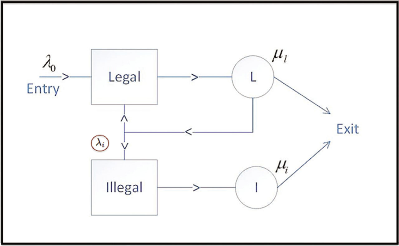
Figure 1
Migration Queuing System (Cases I and II).
In Cases I and II, if migrants are unsuccessful in the legal channel, they can re-enter the legal queue and attempt again or they can enter the parallel illegal QS where acceptance is guaranteed but less-preferred. In Case III, migrants above the quota are diverted automatically to the illegal queue. In each of these stylized cases, migrants are not endowed with personalized attributes. In this respect, a specific QS can refer to a particular category of migrants and there may exist multiple such systems for each type of migrant (e.g., skilled and unskilled). The results in the following cases pertain to how changes in queue parameters influence choices of migrants who share the same observable characteristics. I proceed by using some established results from queuing theory (Medhi [2002]) and perform simple comparative statics analyses where feasible. All three aforementioned cases characterizing stringency in legal migration illustrate the central idea that ceteris paribus, larger flows of illegal migration arise out of greater legal stringency.
2.1. Case I
Assumption 1
Both the legal and illegal queues consist of a Poisson arrival process with parameters λl and λi, respectively. Inter-service times (i.e., time between processing each migrant) are exponentially distributed such that the average intensity of services per unit time are μl and μi, with μl < μi.11
This is denoted in Kendall's notation as an M/M/1 queue where the M stands for Markovian and I restrict attention to a single or centralized server in each channel for simplicity. The average arrival rate of migrants to the legal queue is the sum of the rate of initial entry (λo) and re-entry (λr) into the legal queue, i.e., λl = λo + λr. The corresponding average rate of arrivals to the illegal queue (λi) will be discussed later. This setup also assumes no balking, i.e., once a migrant decides to migrate, she does not leave the QS but only chooses among the two channels and the number of attempts to make in the legal queue.12 Service discipline is first-in-first-out (FIFO).
Now, I define Pn as the probability of there being n people in the QS. In the steady state, the rate up from n to n + 1 people in the queue must be equal to the rate down from n + 1 to n:
where the rate of re-entry is λr = (1 − ν)μl − λi: i.e., the total proportion of migrants who are unsuccessful [(1 − ν)μl] minus the fraction who switch over to the illegal queue (λi). Queuing theory allows us to calculate standard performance indicators, such as the expected number of migrants in the legal QS (refer to Appendix A2).Eq. (2) gives the expected length 〈Q〉 and we can then calculate the expected waiting time 〈Wl〉 of the queue for legal migration.
Assumption 2
The queuing system is stable with positive expected waiting times and queue length. This is contained in the condition holding.
This assumption follows from a technical requirement for the first moments of the queue content (Eq. (2)) and waiting time (Eq. (4)) to be positive and to ensure that the queue is stable, i.e., does not explode. When this is violated, we cannot conduct comparative statics deriving from the stability condition, as the queue increases infinitely. Intuitively, the condition imposes that on average, the traffic in the legal queue must be less than the rate at which migrants exit the QS by being accepted or by switching into the illegal queue.
Migrants have a planning horizon [0,T] and incur a cost C per unit of time that they remain in their origin countries. All migrants are taken to be exponential discounters with a discount rate α. The cost C may be thought of as an opportunity cost or the cost of facing negative circumstances in their home country (such as conflict, unemployment, famine, etc.). The cost is incurred in both legal and illegal queues while the migrant is “waiting” to leave. The cost and discount rate are the same for all migrants in the QS. Benefits from successfully exiting the legal and illegal QS are mRl and Ri per unit of time respectively (Rl > Ri), where m is the maximum number of attempts made to migrate. The key idea behind this requirement is that “something” is gained even from unsuccessful attempts; it may be in the form of experience or know-how about the destination country, which yields higher rewards once the destination is reached. There is no rejection in the illegal QS and all agents are accepted for the journey in their first attempt. Benefits from exiting each queue successfully are the same for all migrants.13
The optimization problem involves choosing the maximum number of attempts (m) the migrant makes to travel legally. The total expected return to a migrant who makes m attempts to migrate legally is the expected return from failing all m times (first term of Eq. (5)) plus the expected return from failing (m − 1) times and succeeding in the mth try (second term of Eq. (5)).14
The first and second-order condition are given in Appendix A4 and evaluating the SOC at the optimum (m*) shows us that it is a local maximum as long as the benefits from migrating legally are high enough relative to the cost of waiting. However, if expected returns from migrating illegally are higher, migrants would switch until the indifference condition is met for the incoming entrant to the system:
where 〈Wl〉 and 〈Wi〉 are the expected waiting times in the legal and illegal QS, respectively, and are both functions of the average rate of arrivals to the illegal queue (λi). Using a queuing theory result, 〈Wi〉 can be calculated in the same manner as before using a similar stability condition specified in Assumption 1.15Next, I use Eq. (6) to examine the comparative statics of how changes in the parameters of the legal queue affect the rate of arrivals (λi) to the illegal queue and summarize them in the form of some results (proofs are in Appendix A5):
Comparative Statics Result 1
Ceteris paribus, increased traffic (ρ) in the legal QS increases the average rate of arrivals (λi) into the illegal QS.
The proof is intuitive; an increase in traffic arises either from more people willing to migrate from the origin country or slower rates of processing migrants legally, both of which increase the expected legal waiting time. Longer waiting periods associated with legal travel are accompanied by higher costs reducing the expected returns from legal migration . To maintain the condition of indifference (Eq. (6)), more migrants would switch over to the illegal channel, increasing the waiting time in the illegal queue.
Comparative Statics Result 2
Ceteris paribus, higher rates of acceptance (ν) in the legal QS lower the average rate of arrivals (λi) into the illegal QS.
This follows from an increase in the expected benefits from legal migration as the chances of getting accepted for travel (ν) increase and the inverse relation between and λi is proved in Result 1. This result is relevant for the role of immigration policy in preventing dangerous and illegal journeys undertaken often with smugglers in periods of mass migration.
The detailed proof in Appendix A5 shows that Result 2 holds as long as the returns from legal entry relative to the cost of waiting is high enough and Figure 2 illustrates this graphically using specific parameter values.16
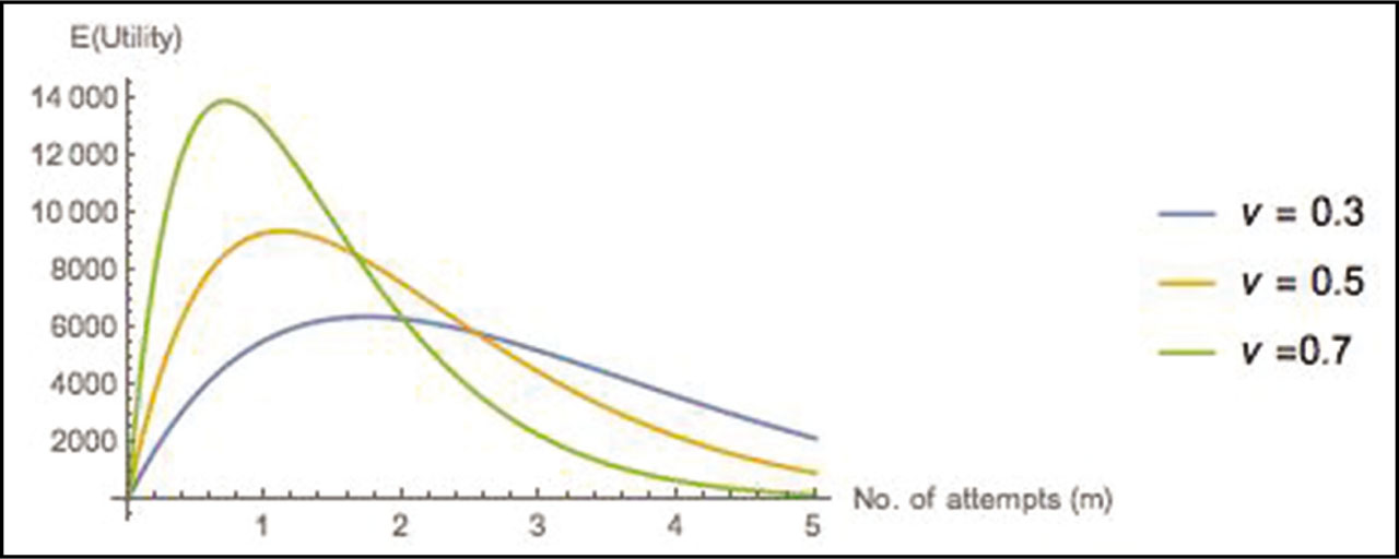
Figure 2
Expected utility from legal immigration at different acceptance rates. Parameter values: Rl = 1000, C =10, α = 0.05, 〈Wl〉 = 4, T = 30.
Comparative Statics Result 3
Ceteris paribus, higher impatience in the form of higher discount rates (α) of the migrants leads to higher average rates of arrival (λi) into the illegal QS.
The intuition behind this proof is that as migrants become more impatient, they are more likely to switch over to the illegal queue. The higher gains from migrating legally would be worth less as they discount the future more. The formal proof given in Appendix A5 rests on precisely this condition that the absolute loss in expected utility from legal immigration due to higher impatience is larger than that for the corresponding loss of expected utility from illegal immigration:
Figure 3 illustrates that the optimal number of attempts (m*) increases as agents are more patient, i.e., have lower discount rates.
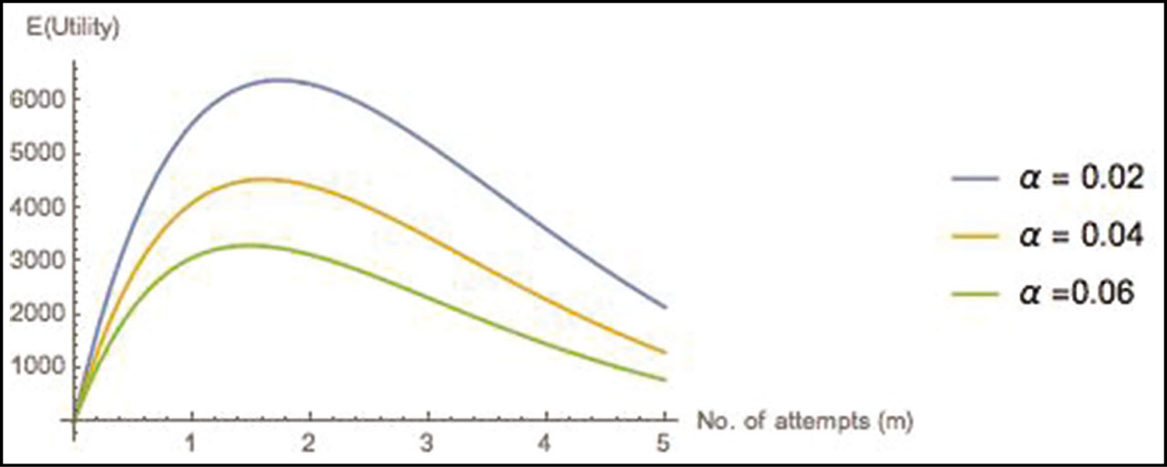
Figure 3
Expected utility from legal immigration at different discount rates. Parameter values: Rl = 1000, C =10, ν = 0.3, 〈Wl〉 = 4, T = 30.
2.2. Case II
Cases II and III illustrate similar findings as Case I but by using different aspects of QS. The previous case considered immigration policy to be comprised of an arbitrary acceptance rate, which is not always realistic. This case expresses the stringency of legal immigration in terms of a minimum waiting time and thereby a minimum cost that the migrant should incur. I assume that this is specified exogenously by the destination country. The waiting time criteria may be thought of as the due diligence towards acquiring the requisite documents, skills, networks, money, etc., necessary for the journey. Alternatively, in case the migrant is in a UNHCR resettlement program, it can be time spent literally waiting in a refugee camp. The limiting criteria, and , lend themselves to immediate analysis. However, a finite is not analytically feasible and I use simulations instead.
The expected return from legal migration after m attempts is:
where | is the indicator function equal to 1 if the migrant has “waited” more than the critical amount specified by the destination country and 0 otherwise. The corresponding expected returns from illegal migration, where there is no minimum criteria, is: where mRl, Ri and C are the homogeneous benefits and waiting cost per unit of time as described earlier, applicable to all migrants.The limiting cases are of no legal criteria: , and infinite legal criteria: . When there are no waiting criteria, success in the legal queue is certain and migrants do not have to make multiple attempts (m = 1). This case is analogous to countries which have open borders with each other (e.g., Schengen member countries). All migrants thus reach their destination legally and an illegal QS does not exist. Expected utility in this case is simply:
where . On the other hand, an infinite waiting period criterion makes it impossible for migrants to legally reach their destination country. A real world example of this is can be cases of “extreme vetting” of citizens from certain countries or immigration from Israel to certain Arab states. In this case all migration is cannibalized by illegal routes and there will be no legal immigration. Returns to illegal migration are as specified in Eq. (10) with the expected waiting time equal to that of a standard M/M/1 queue:2.2.1. Finite legal criteria:
This intermediate case of a finite waiting time criterion is perhaps most realistic and general. It places some “reasonable” bounds on the level of diligence required from the migrant. This diligence may be in the form of actual waiting time or even the time spent in acquiring specific skills which form the basis of immigration – such as for science, technology, engineering, and mathematics (STEM) field workers in the US.17 It is standard for many European countries to explicitly require immigrants to reside within the country and wait a stipulated number of years before getting permanent residency or becoming naturalized or citizens, for example Permit C holders in Switzerland. However, such waiting requirements for accepted asylum status are more nuanced or implicit. The Pew Research Center estimates that the average waiting times for Syrian refugees ranges from 3 months in Germany to more than 1 year in Norway (Connor, 2017). These wait times are not explicit requirements, but depend on processing capacity, origin country, and political pressure on authorities to either accelerate or slow the processing of asylum applications.18 Similarly, in the US, prospective immigrants are faced with different waiting time criteria due to country limits, which cap the number of green cards for any nationality. Under this requirement, immigrants who are applying from China, India, Mexico, and the Philippines, which are at or nearing the country limits, face waiting periods equal to several times that for other nationalities, between 7 years and 23 years (Obinna, 2020).
To model immigration choices under the regime of waiting time criteria, I define a common threshold patience parameter that all migrants are endowed with P = f (α) such that f (α) is a monotonically decreasing function of the discount rate defined in Case 1. This patience parameter represents the maximum number of times a migrant is willing to re-attempt legal migration before switching to illegal routes.19 In this case, it is analytically infeasible to calculate the moments of the queue content and waiting time in the parallel systems. However, a simulation illustrates how queue content varies with and P.
The simulations (Figures 4 and 5) show that:
The relative magnitude of illegal migration increases as the minimum waiting criteria, is increased (from 18 to 40) or the patience parameter, P is decreased (from 4 to 1). The converse is true for the relative share of legal migration.
The queue content exhibits cycles, accumulating and reaching a peak before periodically emptying out once enough potential migrants achieve the minimum waiting criteria.20 This behavior is similar to that of a syphon studied in detail by Filliger and Hongler (2005).
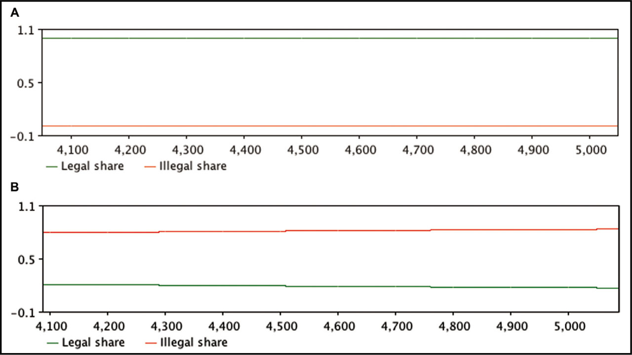
Figure 4
Vertical axis shows steady state relative shares of legal and illegal migration flows and horizontal axis shows time for different patience parameters and critical waiting times.
Source: Simulations using Anylogic Parameter values: λo= 1, μl= 1.4, μi= 1.9 and a) Wlc*= 18, P= 4 (top panel) b) Wlc*= 40, P= 1 (bottom panel).
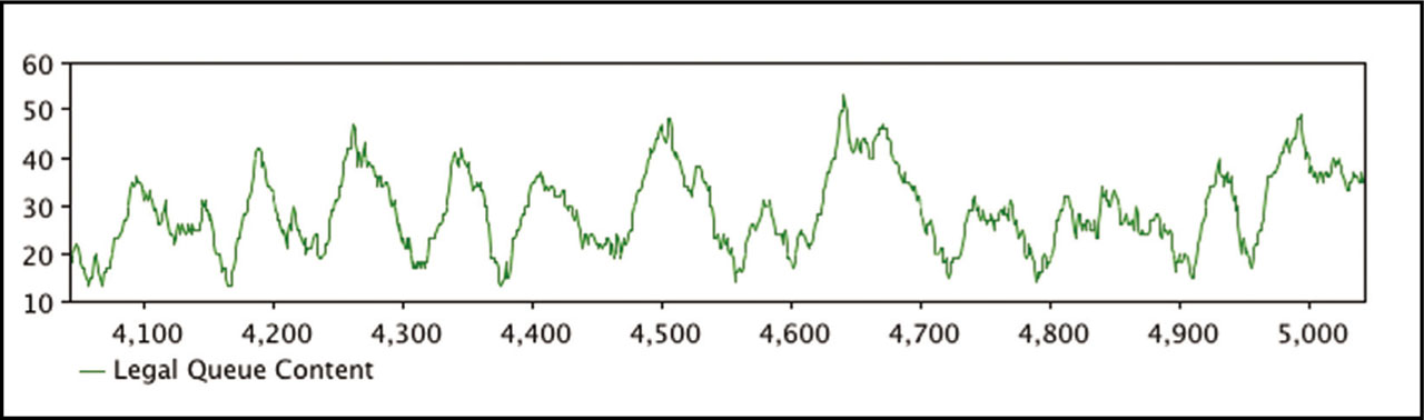
Figure 5
Steady state legal queue content and horizontal axis shows time.
Source: Simulations using Anylogic Parameter values: λo= 1, μj= 1.4, μi= 1.9, Wlc*= 18, P= 4.
2.3. Case III
This case models the stringency of legal channels of immigration in the form of limited waiting area capacity (Figure 6). It is similar to quotas – e.g., those imposed yearly on residence permits and short term permits in Switzerland.21 This is an application of a textbook queuing regime and has been studied in depth by Naor (1969) in the context of imposing tolls to optimize social welfare. The derivations of the QS averages follow similarly with a capacity constraint K (refer to Appendix A3, Case III).
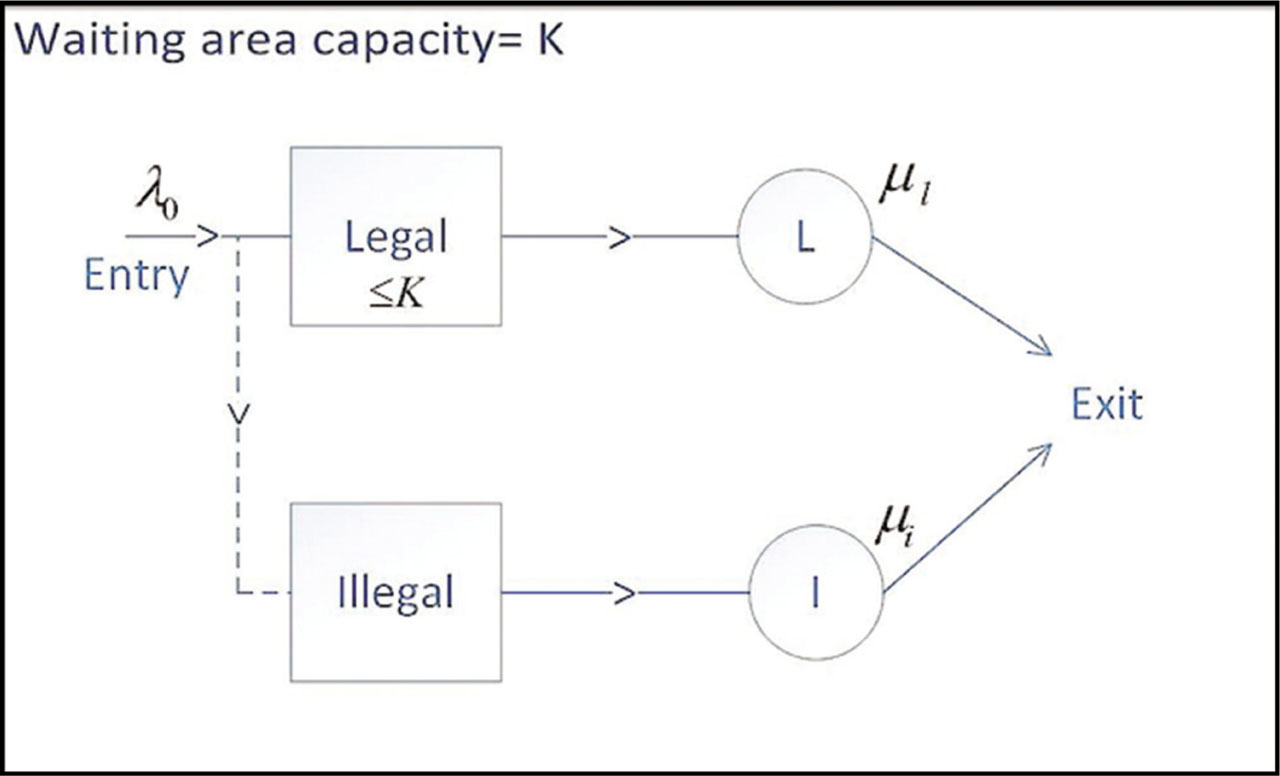
Figure 6
Countries with the highest illegal border crossings over the 5-year period 2010–2014 according to Frontex data.
The analysis is simplified in this case since migrants do not really have a choice about which route to take.22 Both queues operate in parallel with expected returns from legal and illegal migration given below:
andAs expected, an increase in the waiting area capacity (K) decreases the rate of arrivals (λi) into the illegal QS. Refer to Appendix A3, Eq. (19).
Before moving on to the empirical section, I summarize the implications of the theory below:
Given an increase in the number of people attempting to migrate from an origin country and fixed parameters of the legal QS, there will be a spillover into illegal immigration.
Greater stringency in the measures controlling legal immigration, holding the flow of overall potential migrants fixed, would lead to an increase in illegal immigration.
Higher levels of impatience among potential migrants would lead to more “switching- over” to the illegal channel.
3. Empirical Model
Due to the lack of and limitations in existing data, a structural estimation of the model is not feasible. However, I attempt a reduced form analysis to check whether the data contradict the theory of inter-dependent queues of legal and illegal immigration. One major limitation of my data is that it only includes individuals who have successfully reached their destination, legally or illegally. I have no information about the actual number of attempts at migration. Secondly, while the theoretical model consists of agents who are homogeneous in their observable characteristics, no such restriction can be applied to the data.
I use lagged and current values of immigrant flows as indicators of rates of arrival and successful queue completion described in the theoretical section, respectively. Origin-country violent conflict plays a dual role in that it acts as a push for more people to try to migrate and also makes people more impatient to leave (i.e., increases the discount factor α). Regarding impatience, I rely on existing results of Voors et al. (2012), which show that incidences of conflict have the effect of altering individuals’ time preferences, making them more impatient. The dataset refers to immigration into the Schengen region, which is comprised of many different countries; so, destination-country immigration policy is hard to capture. Year fixed effects are included to control for changes that occur at the Schengen region level.
Thus, the two main effects I look for in the data are of origin-country shocks of conflict and inter-QS effects. The equations to be estimated are:
where the dependent variable kit and its lag refer to the log of IBCs into the Schengen region from country i in year t, and lit the corresponding log of inflow of documented or legal migrants.23 The variable cit−1 refers to the log of conflict-related deaths occurring 1 year prior to the year of migration. The lag is used to account for the fact that migration requires preparation or waiting time before the journey can be undertaken. Relevant covariates (xit) and year (λt) and country (αi) specific fixed effects are included. ɛit and ηit are the pure error terms.3.1. Data sources
Available data on the EU refer to migrants who have successfully, either legally or illegally, entered the EU. The data on the inflow of migrants with legal status are from Eurostat, the statistical office of the EU. These data are disaggregated by country of citizenship and are available yearly. The definition of a “legal migrant” varies from country to country.24 Schengen countries usually require an actual or intended stay of 12 months and report the data to Eurostat from population registers, administrative records, and national surveys.
Frontex records the number of detected IBCs via land and sea routes into the Schengen region. Disaggregated data by nationality are available from the 3rd quarter of 2007 and are updated monthly.25
Figure 7 shows the evolution of IBCs from the six countries with the highest flows over 2010–2014 period. Pursuant to eyeballing the panels for Tunisia and Syria, we are presented with a sharp peak for the months immediately following their respective domestic conflicts.
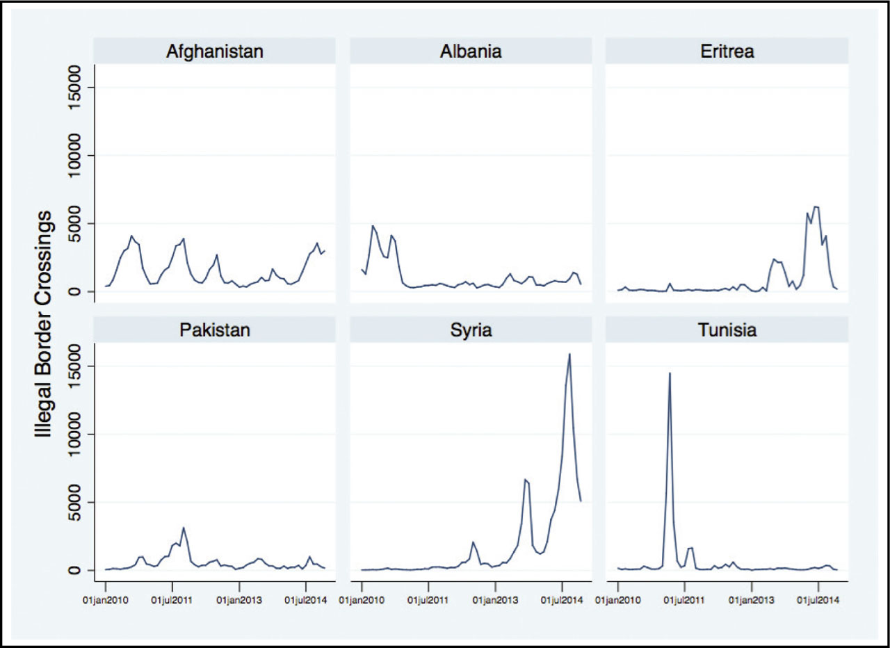
Figure 7
Migration Queue (Case III).
Source: Author's representation.
For data on conflict, I use the Georeferenced Event Dataset (GED) from the Uppsala Conflict Data Program (UCDP version 17.1 2017). An event is an incident where armed force was used by an organized actor against another organized actor, or against civilians, resulting in at least one direct death at a specific location and a specific date. The UCDP dataset records three values for the number of conflict-related deaths: a low, high, and a best estimate. All estimates are sourced from publicly available and reliable information and are collected at the level of town and village for urban and rural areas respectively. For this paper, I collapse the data to the country level. The UCDP GED dataset does not yet include deaths from Syria as data collection is not complete at the granular level of towns and villages. I include Syria by using the conflict level data from the UCDP Battle-related Deaths (BRD) dataset.26
My sources for other relevant covariates are the World Development Indicators (WDI) for population density and World Governance Indicators (WGI) for institutional quality.27 Complete data from all sources is available from 2008 to 2015; so, I restrict attention to this time period. Thus, I have a strongly balanced panel dataset with 8 years and 137 origin countries for IBCs and 218 origin countries for legal inflows. I transform all the above variables using the inverse hyperbolic sine transformation, except the institutions score to address the presence of a long right tail and zeros in the data.28 Summary statistics of the relevant variables are presented in Table 1.
Table 1
Summary statistics
| Variable name | Category | Mean | Standard deviation | N | AR(1) Coefficient | |
|---|---|---|---|---|---|---|
| Log legal inflow | Overall | 5.808 | 2.888 | 1,744 | 0.177 | 0.97 |
| Between | 2.854 | 218 | ||||
| Within | 0.478 | 8 | ||||
| Log illegal inflow | Overall | 3.479 | 3.257 | 1,096 | 0.296 | 0.81 |
| Between | 3.092 | 137 | ||||
| Within | 1.052 | 8 | ||||
| Log CD | Overall | 1.115 | 2.466 | 1,768 | 0.309 | 0.68 |
| Between | 2.241 | 221 | ||||
| Within | 1.039 | 8 | ||||
| Log CD difference | Overall | 0.800 | 2.025 | 1,768 | 0.230 | 0.71 |
| Between | 1.800 | 221 | ||||
| Within | 0.934 | 8 | ||||
| Log GNI per capita | Overall | 9.871 | 1.246 | 1,274 | 0.781 | 0.96 |
| Between | 1.211 | 188 | ||||
| Within | 0.077 | 6.8 | ||||
| Log population density | Overall | 5.097 | 1.567 | 1,644 | 0.965 | 0.98 |
| Between | 1.568 | 206 | ||||
| Within | 0.046 | 8 | ||||
| Institutions score | Overall | −0.033 | 0.995 | 1,592 | 0.636 | 0.91 |
| Between | 0.990 | 200 | ||||
| Within | 0.138 | 8 |
[i] Note: AR(1) coefficients and the relative variance explained by fixed effects are calulated by estimating yit = ρyit−1 + αi + ɛit.
[ii] CD, conflict deaths.
3.2. Identification strategy
The parameters of interest are the β′s and γ′s of Eqs (15) and (16). Due to potential endogeneity and the dynamic panel setting, I use a GMM approach to estimate the coefficients of interest using internal as well as external instruments. The external instrument to consistently estimate the effect of conflict arises from the dataset itself. The UCDP dataset records three values for the number of battle related deaths: a low, high, and a best estimate. The estimates are collected from third parties such as news agencies, international and non-governmental organizations. In addition, the sources also include reports from the warring parties themselves (governments and opposing groups). Due to the difficulties in accessing accurate information during a violent conflict and the vested interests of governments or opposition parties in releasing accurate fatalities, there are discrepancies regarding the exact number of conflict-related deaths. This is even greater when conflicts are spread out geographically over a region, some locations of which are inaccessible. The discrepancies, measured by the difference between the high and the low estimate, are positively and strongly correlated with the level of the best estimate, thereby satisfying the criterion of instrument relevance. This should be unsurprising as it is harder for independent reporters or watchdogs to access locations during conflicts occurring at a massive scale (Themnér and Wallensteen, 2014).29
The second criterion of the exclusion restriction is more complicated to support. The difference in the high and low estimates of death may actually be picking up the nature of institutions instead of the intensity of the conflict itself. To account for this, I control for the quality of institutions in the country by using the rule of law indicator. Further, if we consider the group of countries which have no discrepancies in the measurement of deaths in the presence of violent conflict, their mean score on the institutions indicator is negative (−0.61), which is clearly a counter to the argument that the instrument is picking up institutional quality.
In this dynamic panel setting of lagged effects and in the absence of sufficient external instruments, I use a GMM approach to exploit all available moment conditions using internal instruments. Due to the possibility of persistence and the high relative share of variance in fixed effects , the first-differenced GMM estimates may suffer from poor finite sample properties, namely bias and imprecision, since lagged levels are weak instruments for first-differences (Blundell and Bond, 2000). Hence, I estimate the model using system GMM, which estimates the model using the equations in levels and differences to improve the strength of internal instruments. Lastly, another issue potentially compounding the endogeneity problem is the possibility of serially correlated errors. This is addressed by the common factor representation below given by Blundell and Bond, 2000 and also implemented by Arcand et al. (2008).
Results using the above estimation techniques are presented in the next section.
4. Results
I focus first only on the effect of conflict and omit the lagged legal and illegal inflows from the right-hand side of the model. Results using pooled Ordinary Least Squares (OLS) and within-estimators are given in Tables 2 and 3. The significance of the positive conflict coefficient remains for IBCs after introducing controls and fixed effects but not for legal inflows. In Column 4 of Tables 2 and 3, I restrict the sample to only those countries with any present or past incidences of conflict within the panel length, to explore further the relationship between the two migration variables and conflict. The significance of the positive conflict coefficient remains for IBCs but not for legal inflows. This illustrates that the relationship between conflict and illegal migrant flows is not driven solely by the differences between countries that experience violent conflict and those that do not.
Table 2
Pooled OLS and within-estimator dependent variable: Illegal inflow
| OLS | Within | Within | Within | |
|---|---|---|---|---|
| All | All | All | Restricted sample | |
| (1) | (2) | (3) | (4) | |
| Log CDt−1 | 0.306*** (0.035) | 0.094** (0.040) | 0.082** (0.038) | 0.071* (0.036) |
| Log population density | 0.244*** (0.050) | 6.761*** (2.571) | 4.234 (3.394) | |
| Institutions | −1.390*** (0.095) | −0.813 (0.579) | −1.419** (0.672) | |
| Constant | 0.887*** (0.336) | 2.987*** (0.130) | −29.881** (12.270) | −17.052 (15.764) |
| Year fixed effects | Yes | Yes | Yes | Yes |
| Country fixed effects | Yes | Yes | Yes | |
| Adjusted R2 | 0.273 | 0.130 | 0.171 | 0.246 |
| Number of observations | 920 | 959 | 920 | 497 |
| Number of countries | 137 | 132 | 71 |
Table 3
Pooled OLS and within-estimator dependent variable: Legal inflow
| OLS | Within | Within | Within | |
|---|---|---|---|---|
| All | All | All | Restricted sample | |
| (1) | (2) | (3) | (4) | |
| Log CDt−l | 0.302*** (0.016) | 0.033 (0.034) | −0.000 (0.011) | −0.009 (0.012) |
| Log population density | −0.231*** (0.056) | 0.648 (0.562) | 0.599 (0.685) | |
| Institutions | 0.268*** (0.071) | 0.000 (0.196) | −0.450** (0.176) | |
| Constant | 6.905*** (0.321) | 5.556*** (0.062) | 2.943 (2.796) | 4.008 (3.306) |
| Year fixed effects | Yes | Yes | Yes | Yes |
| Country fixed effects | Yes | Yes | Yes | |
| Adjusted R2 | 0.101 | 0.039 | 0.054 | 0.142 |
| Number of observations | 1,364 | 1,526 | 1,364 | 532 |
| Number of countries | 218 | 196 | 76 |
Now, given that there are endogeneity issues, most obviously due to omission of lagged inter-queue variables, the coefficients in Tables 2 and 3 are likely to be inconsistent. As mentioned in section 4.2, I use the difference between the high and low estimates of conflict deaths (CD) as an Instrumental Variables (IV) for its best estimate. This is driven by strong correlation between the level of discrepancy and the level of the conflict itself. Controlling for the quality of institutions, as measured by the rule of law indicator, this discrepancy should not be related to immigration in any other way.
Using the difference between high and low estimates of CD as an IV, Table 4 shows that lagged conflict in origin countries positively affects IBCs but has no effect on the legal inflow of migrants into Schengen countries. The coefficient for conflict is relatively stable across specifications. There is a strong mechanical correlation between the IV and the endogenous conflict variable (refer to Table 4, Part B). This “relevance” of the difference in high and low estimates of CD to its best estimate is because for observations which have no conflict, the difference in estimates is also equal to zero. Thus, I restrict the sample to only those countries which see any present or past incidences of conflict within the panel length (Columns 3 and 6, Table 4) and find that the result still holds. The strength of the instrument does not rely on mechanical relevance alone (Columns 3 and 6, Table 4 Part B).
Table 4
Two-Stage Least Squares (2SLS) estimator
| Part A | Legal inflow | Illegal Inflow | ||||
|---|---|---|---|---|---|---|
| All | All | Restricted sample | All | All | Restricted sample | |
| (1) | (2) | (3) | (4) | (5) | (6) | |
| Log CDt−1 | 0.042* (0.022) | −0.000 (0.013) | −0.010 (0.013) | 0.120*** (0.039) | 0.120*** (0.041) | 0.106** (0.041) |
| Log population density | 0.648 (0.410) | 0.600 (0.499) | 6.783*** (1.610) | 4.162** (2.111) | ||
| Institutions | −0.000 (0.154) | −0.453*** (0.130) | −0.724* (0.371) | −1.288*** (0.458) | ||
| Year fixed effects | Yes | Yes | Yes | Yes | Yes | Yes |
| Country fixed effects | Yes | Yes | Yes | Yes | Yes | Yes |
| Part B | First stage dependent variable: Log CD | |||||
| Log CD difference | 0.828*** (0.041) | 0.800*** (0.044) | 0.782*** (0.045) | 0.824*** (0.040) | 0.789*** (0.043) | 0.779*** (0.043) |
| Log population density | 0.628 (0.796) | 3.522* (1.944) | 1.133 (1.130) | 3.289* (1.995) | ||
| Institutions | −0.576*** (0.178) | −1.831*** (0.454) | −1.096*** (0.316) | −1.811*** (0.462) | ||
| Number of observations | 1,526 | 1,364 | 532 | 959 | 920 | 497 |
| Number of Countries | 218 | 196 | 76 | 137 | 132 | 71 |
| Kleibergen-Paap F-stat | 405.913 | 327.501 | 302.436 | 430.805 | 340.704 | 322.067 |
Finally, I turn to the complete model (Eqs (15) and (16)), which includes the inter-queue effects.30 Table 5 uses lags t − 1 to t − 3 of endogenous variables as instruments and the external instrument mentioned earlier. All estimates are calculated using the two-step covariance matrices along with the finite-sample correction given by Windmeijer (2005), which makes two-step robust estimations more efficient in small T large N datasets. However, the results presented in Columns 5 and 6 of Table 5 use the one-step covariance matrix and the findings are not robust to the two-step covariance matrix estimation.
Table 5
GMM estimates
| Difference GMM | System GMM | Common factor | ||||
|---|---|---|---|---|---|---|
| Illegal | Legal | Illegal | Legal | Illegal | Legal | |
| (1) | (2) | (3) | (4) | (5) | (6) | |
| Log illegal inflowt−1 | 0.103 (0.085) | −0.030 (0.030) | 0.752*** (0.047) | 0.018 (0.012) | 0.806*** (0.047) | −0.008 (0.016) |
| Log illegal inflowt−2 | 0.027 (0.016) | |||||
| Log legal inflowt−1 | −0.105 (0.152) | −0.140* (0.074) | 0.266*** (0.085) | 0.899*** (0.031) | 0.050 (0.088) | 0.903*** (0.027) |
| Log legal inflowt−2 | 0.163** (0.081) | |||||
| Log CDt−1 | 0.010 (0.059) | −0.009 (0.020) | 0.071** (0.034) | 0.013 (0.011) | 0.063** (0.032) | 0.002 (0.013) |
| Log CDt−2 | 0.015 (0.031) | 0.008 (0.015) | ||||
| Year fixed effects | Yes | Yes | Yes | Yes | ||
| Number of observations | 804 | 804 | 938 | 938 | 804 | 804 |
| Number of countries | 134 | 134 | 134 | 134 | 134 | 134 |
| Number of instruments | 46 | 46 | 71 | 71 | 73 | 73 |
| AR(1) p-stat | 0.0004 | 0.1682 | 0.0000 | 0.0000 | 0.0000 | 0.0000 |
| AR(2) p-stat | 0.1811 | 0.7931 | 0.3345 | 0.0821 | 0.4006 | 0.1477 |
| Hansen p-statistic | 0.0004 | 0.0574 | 0.0194 | 0.0645 | 0.0085 | 0.0601 |
From Table 5, there is evidence of positive spillovers from legal immigration flows on illegal flows but none in the opposite direction. There is also evidence of persistence of own queue effects. The previous results regarding the effect of conflict related deaths still hold, in that they positively affect illegal immigration flows and have no effect on legal flows.
4.3. Additional results
One drawback of the above results is that it does not account for the inherent differences between people attempting to migrate legally compared to those who do so illegally. Documented migration to Europe usually occurs under the following categories – remunerated activities, family reunification, education and humanitarian reasons. Differences within individuals from the same country would make some people more eligible to meet these criteria than others. Since I do not have data on individual level characteristics, I cannot control for them. However, the theory in Section 3 implies that given the same characteristics of individuals, migrating via the legal queue is likely to involve larger waiting costs that lead some people to switch over to the illegal channel. Looking at the effect of violent conflict on the flows of legally resettled people who might share similar characteristics within the origin countries gives evidence to these waiting costs.
“Resettlement is one tool to help displaced persons in need of protection reach Europe safely and legally, and receive protection for as long as necessary. It is a durable solution which includes selection and transfer of refugees from a country where they seek protection to another country” EPRS, 2017. The UNHCR has to determine whether an applicant is a refugee according to the 1951 Geneva Convention, and has to identify resettlement as the most appropriate solution. From Table 6 we see that the relationship between violent conflict and the magnitude of resettled persons is not very robust within the dataset available. Only the third lag of CD is significant using the within estimator and this significance becomes weaker after introducing other covariates. The same goes for results from 2SLS estimation using the difference in estimates of CD as an IV for CD.
Table 6
Within and 2SLS estimators dependent variable: Log of resettled persons
| Within | Within | Within | Within | 2SLS | 2SLS | |
|---|---|---|---|---|---|---|
| (1) | (2) | (3) | (4) | (5) | (6) | |
| Log CDt−1 | 0.072 (0.048) | |||||
| Log CDt−2 | 0.072 (0.045) | |||||
| Log CDt−3 | 0.130*** (0.048) | 0.077* (0.046) | 0.143** (0.066) | 0.068 (0.066) | ||
| Log population density | −1.059 (2.129) | −1.085 (2.131) | ||||
| Institutions | −0.400 (0.328) | −0.407 (0.332) | ||||
| Constant | 0.617*** (0.102) | 0.674*** (0.087) | 0.464*** (0.096) | 5.755 (10.530) | 0.445*** (0.118) | 5.896 (10.538) |
| Year fixed effects | Yes | Yes | Yes | Yes | Yes | Yes |
| Country fixed effects | Yes | Yes | Yes | Yes | Yes | Yes |
| Adjusted R2 | 0.013 | 0.012 | 0.036 | 0.017 | ||
| Number of observations | 1,576 | 1,379 | 1,182 | 952 | 1,182 | 952 |
| Number of groups | 197 | 197 | 197 | 192 | 197 | 192 |
5. Discussion
This paper is addressed to two broad audiences. The first audience comprises of development economists who are working on immigration and would be interested in alternative frameworks to study mass migration and crises therein. The second audience includes those economists who work on stochastic processes and specifically, queuing theory, who would be interested in its application to real-world phenomenon such as migration. This paper provides a stylized model focusing on how migration crises emerge out of linkages between legal and illegal channels of entry and the dynamic nature of the same. However, it has several limitations. Firstly, it does not account for migrant heterogeneity and this is one research area with great potential for future work.31 Secondly, the current framework is restrictive in that it does not allow for complete breakdowns of migration control services as we have witnessed in the recent past. Under such circumstances of discontinuity, massive flows would, in fact, drive costs of illegal migration further down. Despite these limitations, this baseline illustrates how the migration choices of others may influence individual decisions beyond a certain threshold level of traffic.
Empirically, this paper attempts to study the effect of conflict on different channels of immigration. To the my knowledge, this has not been addressed as yet in the context of the recent crisis and particularly, has not made use of the Frontex dataset on IBCs into the Schengen region. While I cannot estimate the full structural model and the panel length of the data is only 8 years, the results show clearly the one-way inter-queue effects spilling over from legal to illegal flows and the lack of sensitivity of legal immigration to origin-country shocks such as conflict. It is however quite possible that the short length of the panel does not allow these effects to show up – but that is precisely support for the frictions that the theory assumes.
Although much attention has been given to South–North migration in the media, North–North and South–South migration together account for a majority (59%) of global immigration with South–South migration having the largest share (UNDESA, 2013). Crisis-like scenarios regarding South–North migration emerge due to the rigidity and slow-moving nature of legal processes of resettlement and assessment of asylum applications. A role for future research would be to shed light on immigration policies that account for inter-linkages between different channels instead of addressing individual channels as systems in isolation.
Declarations
Availability of data and material
All data used in this paper are publicly available and can be found in the sources provided in the Data Sources section. Links are listed below.
Data on legal immigration flows are from Eurostat downloadable at: https://ec.europa.eu/eurostat/data/database
I received data from Frontex on IBCs via email but they are now publicly available at: https://data.europa.eu/euodp/en/data/publisher/frontex
Conflict data is from UCDP is downloadable at: https://ucdp.uu.se/downloads/
Covariates are from WDI and available at: https://datacatalog.worldbank.org/dataset/world-development-indicators
Competing interests
Not applicable.
Funding
Not applicable.
Acknowledgements
This paper was a part of my doctoral dissertation and I am indebted to Jean-Louis Arcand, Shantayanan Devarajan, Slobodan Djajić, Max-Olivier Hongler, Sripad Motiram, Guillaume Sartoretti and Shekhar Hari Kumar for their invaluable comments and help on this paper.
Appendices
Appendix
A1. General derivations
The results in this section are of standard M/M/1 queues and draw extensively from Medhi, 2002.
Arrival process: Arrivals are distributed by the Poisson distribution with parameter λo, which implies exponential inter-arrival times. The derivation for the average inter-arrival time is given below. The average rate of arrivals is just the inverse of that.
Service process: The time between consecutive services is distributed exponentially. The derivation of average inter-services is given below. The average rate of services is the inverse of that.
A2. Case I queue performance indicators
Thus, the stability condition from Eq. (1) is:
By the normalization condition we have:
Using the Moment Generating function:
A3. Case III: Maximum capacity (K)
We start with the steady state equation again:
Using the generating function as before, the expected number of migrants E (Ql) in the legal queue is:
To calculate the expected waiting time, the effective rate of entry (λ′) is used, given that the QS has not reached capacity yet:
A migrant upon being diverted from the legal channel will join the illegal QS. In this case, the illegal channel of migration is used only when the legal waiting area is at its capacity; the rate of arrival (λi) into the illegal QS depends on the legal QS operating at capacity.
So, average illegal queue length is given by:
similarly, using Little's LawA4. Case I - First- and second-order conditions
Migrants maximize expected utility with respect to the maximum number of attempts they make for legal entry (Eq. (5) rewritten below).
Further, the FOC w.r.t. m is given below:
Differentiating with respect to m again and evaluating at the optimum m* gives:
Rearranging terms gives:
Analysis of above terms show that the expression for the second-order condition is negative as long as the benefit from legal migration is large enough, and specifically if . This implies a local maximum at m*.
A5. Proofs
Result 1
Ceteris paribus, increased traffic (ρ) in the legal QS increases the average rate of arrivals (λi) into the illegal QS.
Proof
This follows from an increase in expected waiting time in the legal QS, 〈Wl〉, which lowers . Subsequently, more migrants would switch to the illegal QS. The first two parts of the claim are straightforward from Eqs (4) and (5).
Next I use Eq. (6) to show the inverse relationship between λi and . Define
Result 2
Ceteris paribus, higher rates of acceptance in the legal QS lowers the average rate of arrivals (λi) into the illegal QS.
This follows from an increase in as (ν) increases and the inverse relation between and λi proved above. Thus, the proof follows from differentiating Eq. (5) with respect to ν.
The first term of Eq. (20) is positive and the second term is also positive if the following condition holds:
Result 3
Ceteris paribus, higher impatience in the form of higher discount rates (α) of the migrants leads to higher average rates of arrival (λi) into the illegal QS.
Proof
This follows from Eq. (6) and a result from Result 1.
where the denominator from Result 1. Thus what remains to be shown is that the numerator is negative. which holds if the absolute loss in expected utility from legal immigration due to higher impatience is larger than that for the corresponding loss of expected utility from illegal immigration: