
I. Introduction
Early recognition and identification of motor faults, which can be broadly segmented into mechanical and electrical, is essential in order to guarantee the reliability and economic operation of the motor. Common fault detection and diagnosis (FDD) techniques are commonly divided into three different paradigms: signal-based, model-based, and knowledge-based. Model-based techniques are exploited to produce analytical representations developed from physical principles and system identification, but they will become less and less viable with the growing complexity of systems. By contrast, signal-based methodologies focus on the measurement of many, various, measurable quantities—such as vibration, motor current, rotational speed, and temperature—to find out and characterize the fault. Popular signal processing methods used to detect electrical machinery faults include spectral estimation [1,2], time–frequency analysis [3], fast Fourier transform [4,5,6], scale-invariant feature transform [7], sequence analysis [8], and wavelet transformation and decomposition [6,7,8]. These approaches rely on advanced signal processing frameworks that can generate salient features from the raw data, which help to determine the anomalies associated with the problem (i.e., bearing defects).
Unlike classical methodologies, data-driven condition monitoring schemes are being built on the high data content collected by advanced sensing, data acquisition, and control systems. In this domain, shallow machine learning models have been shown to be capable of detecting and diagnosing fault-specific motor current signals [9]. However, they often use features crafted by hand, and diverse classifiers, frequently fed short data sets of specific motors or rotating machinery (RM). Therefore, their usability is limited, and their performance declines with a variety of system types, fault states, or larger datasets, which makes developing a universal diagnosis system quite difficult. An excellent example of this limitation is the presence of variability in fault detection for machines powered by adjustable speed drives that operate under varying speeds, adding the challenge of robust fault diagnosis.
II. Related Work
Feature extraction is an important aspect of fault diagnosis in that it is used to identify and describe informative patterns from raw data, that is, vibration signals, to make fault diagnosis more accurate. Traditional feature extraction methods, such as empirical mode decomposition (EMD), symbolic aggregate approximation, and multifractal analysis, have been widely used in the domain of RM diagnostics. For example, [10] introduced the EMD-based method, based on which extracted features were proposed to intelligently find the faults for the rotating mechanism using a non-naive Bayesian classifier. Similarly, [11] used a symbolic aggregate approximation frame-work to extract features from bearing vibration signals and categorize the features with the nearest neighbor algorithm. On the other hand, [12] showed that bearing vibration signals have multifractal characteristics, and they motivated researchers to utilize multifractal detrended fluctuation analysis to extract features for proactive fault detection. Additionally, [13] proposed to alleviate the drawbacks of the classical Fourier-based methodologies through continuous wavelet transform for signals, including support vector machines (SVM) for fault classification.
Traditional feature extraction methods have been successful at fault diagnosis. Currently, these methods largely use shallow learning approaches, which have their own limitations. Methods such as Bayesian classifiers, nearest-neighbor methods, and SVMs require manual feature engineering. Because we need this knowledge in classifiers, they tend to be very time-consuming and dependent on expertise in the domain. For instance, the performance of these classifiers is highly contingent upon the quality of the extracted features, resulting in an often-arbitrary selection of features as well as substantial risk of human error. In addition, shallow learning methods tend to be unable to capture complex non-linear relations, especially for high-dimensional and noisy signals. Recent deep learning models, such as convolutional neural networks (CNNs) and recurrent neural networks (RNNs), have been of great interest for their ability to learn hierarchical features independently from raw data automatically by avoiding the necessity of manual feature engineering [14]. They effectively process big data, discover complex patterns, and can adapt under variable conditions, improving their robustness and scalability when applied to fault diagnosis. Nevertheless, despite its benefits, deep learning techniques require huge amounts of computational resources and extensive labeled datasets for effective training and can pose problems in specific industrial settings.
Several data-driven deep neural network (DNN) models have been proposed in the literature for the problem of FDD. DNNs possess the capability to automatically learn discriminative features directly from raw input data during the training process, thereby eliminating the reliance on manually engineered statistical or transform-domain feature representations. While this improvement is particularly advantageous, the approach of such models depends significantly on access to large, correctly labeled datasets, which is crucial for efficient training and generalization.
To combine computational efficiency and diagnostic performance, a number of works [15,16,17] have used one-dimensional (1D) CNNs to diagnose machinery faults with either raw signals or pre-extracted features under fixed operating conditions. Although these 1D CNNs have obtained promising performance in such controlled conditions, previous studies [18,19] indicated that CNNs built with standardized architecture following first-order neuron models commonly fail to capture the complexity of highly non-linear solution spaces. As a result, such models typically require more network depth and architectural complexity, which are critical components of satisfactory performance on more challenging fault diagnosis tasks.
The following are the three main contributions based on the methods and results described in the paper.
Hybrid CNN-transformer design: We introduce FaultFormer-Net as a hybrid deep learning frame-work consisting of a CNN and a transformer encoder for local temporal feature extraction and long-range temporal dependencies. Such a structure can easily capture transient vibrations and the periodic faults observed in bearing signals.
Multi-domain feature fusion approach: We build a multi-domain feature fusion architecture that merges the deep-learned representations with handcrafted time-domain statistical descriptors and frequency-domain spectral features for the unified vector representation. This integration increases the model's discriminative accuracy and maintains physical interpretability of vibration signal properties.
The highest levels of diagnostic accuracy and strength: The model demonstrates 99.98% classification accuracy, 99.68% of precision and recall, while achieving 99.80% of F1-score on the bench-mark Case Western Reserve University (CWRU) bearing dataset, which is superior to several state-of-the-art algorithms proposed recently. It also shows robustness across 10 bearing fault categories, including varying motor loads (0–3 hp), to ensure that it is a very reliable model for industrial condition monitoring.
III. Material and Method
a. Dataset description
The CWRU bearing dataset (https://www.kaggle.com/datasets/brjapon/cwru-bearing-datasets) is one of the most commonly used benchmark datasets to evaluate bearing fault diagnosis algorithms in RM. It was created by CWRU's bearing data center to study and investigate machine condition monitoring and fault detection topics. In-house data is collected using a motor-driven mechanical system, consisting of a 2 hp induction motor, a torque transducer, and a dynamometer. Accelerometers mounted on the drive end (DE) and fan end (FE) of the motor housing were used to detect vibration signals created with variations in operation. Since bearing faults vary over time, vibration signals were sampled at high frequencies (usually 12 and 48 kHz) to reflect the characteristics of the bearing faults accurately.
To model an actual fault in a bearing, problems were manufactured in the bearings by means of electrical discharge machining. The dataset contains various fault types, such as inner race faults, outer race faults, rolling-element (ball) faults, and normal (healthy) bearing conditions. These faults were generated with different sizes of defects (e.g., 0.007, 0.014, and 0.021 in.) to depict the types of fault severities. Moreover, the works were performed at various motor loading conditions (0, 1, 2, and 3 hp), corresponding to rotating speeds from approximately 1797–1720 rpm. Given this divergence in operating regimes, it is possible for researchers to assess the robustness of diagnostic algorithms at various mechanical loads. Because of its well-organized fault categories, high-quality vibration measurements in controlled experimental environments, and controlled experimental conditions, the CWRU dataset has been developed as a benchmark for validating both classical machine learning techniques and modern deep learning-based fault diagnosis frameworks.
b. Methodology
We introduce a hybrid intelligent framework, shown in Figure 1, for automatic rolling bearing fault diagnosis through vibration signals. Our proposed method combines signal preprocessing, statistical feature extraction, deep feature learning from a CNN-transformer architecture, frequency-domain analysis, and classification based on a DNN.
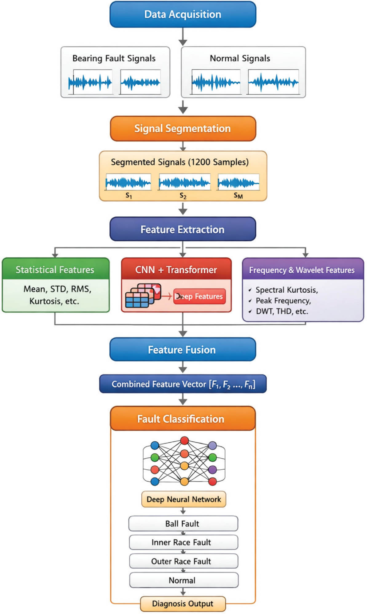
Figure 1:
The proposed FaultFormer framework for induction motor bearing faults classification. CNNs, convolutional neural networks; RMS, root mean square.
The proposed framework achieves a combination of handcrafted signal features with deep representations, captures physical signal characteristics and high-level latent features, providing robust classification of multiple bearing fault conditions. The workflow of the proposed system, shown in Figure 1, has five key stages: data acquisition, signal segmentation, feature extraction, feature fusion, and fault classification.
b.i. Data acquisition
The vibration signals used in this study derive from the CWRU bearing dataset, which is widely recognized as a benchmark dataset for bearing fault diagnosis research. The dataset contains vibration measurements recorded using accelerometers mounted at the DE and FE of an induction motor. These measurements correspond to different bearing health conditions, including ball faults, inner race faults, outer race faults, and normal operating conditions.
Let the vibration signal acquired from the accelerometer be represented as
where xi represents the vibration amplitude at the ith sampling instant and N denotes the total number of samples in the signal.Since the dataset contains signals of varying lengths, the minimum signal length among all classes is determined to maintain uniformity during analysis. This is given by
where k denotes the total number of fault conditions. Selecting the minimum signal length ensures balanced data representation and avoids bias during feature extraction.b.ii. Signal segmentation
The raw signals are split into fixed-length segments to catch localized characteristics of vibration signals. Signal segmentation is an important part of preprocessing that helps increase the number of training samples, and thus improve the robustness of feature extraction. Each vibration signal is divided into segments of length L = 1200 samples, which corresponds to vibration data around 0.025 s.
Thus, the jth segment can be expressed as
Where sj represents the jth signal segment, L denotes the segment length, and j = 1,2,...,M, where M is the total number of segments.
There are multiple advantages to segmenting the vibration signals. It enables to obtain transient fault patterns, which can occur in very short time periods. It extends the data samples available and thus boosts the training performance of machine learning models. Segmentation finally enables the extraction of localized statistical and spectral features.
b.iii. Statistical feature extraction
Time-domain statistical characteristics are a valuable source of information for amplitude distribution and variation of the vibration signal. Such terms are frequently used during the operation of condition monitoring systems due to their ease and power in picking out fault-induced anomalies.
Quantitative statistical parameters are an essential property of vibration-based fault diagnosis, as they convey short and numerical interpretations of signal behavior in the time domain. Such features give a summary of complex vibration patterns (using a limited number of parameters), allowing effective differentiation in normal and faulty operating conditions. Physical faults, including bearing defects, induce impulse shocks as well as varying vibration patterns, which are evident through statistical changes in mean, standard deviation, root mean square (RMS), skewness, and kurtosis. For example, kurtosis and crest factor are very sensitive to abrupt impulses caused by localized defects, and thus can be employed as a useful parameter for monitoring early faults.
The second key benefit of statistical features is that they are computationally low and are extremely physically interpretable. Statistical measures allow for simplifications and computational methods to be applied to raw vibration data, and thus can be applied directly to the output signals of industrial sensors, while advanced signal processing tools need to perform complicated transformation-based functions. Furthermore, the statistical parameters each represent a physical property corresponding to a particular vibration signal, such as energy content, variability, or impulsiveness, and are useful for engineers to understand the state of the machine. Combined with deep learning and the frequency domain features, statistical descriptors improve the general robustness of a fault diagnosis framework and its discriminating ability. Several statistical descriptors shown in Table 1 are calculated for each signal segment.
Table 1:
Statistical features
| Sr. No. | Feature | Mathematical Expression | Advantage |
|---|---|---|---|
| 1. | Maximum & Minimum amplitude | Indicators of mechanical impacts | |
| 2. | Mean | Average vibration level | |
| 3. | Standard Deviation | Indicate increased vibration fluctuations associated with faults | |
| 4. | Root Mean Square | Analyzing vibrations. An indicator of the severity of mechanical faults. | |
| 5. | Skewness | Sensitive to impulsive behavior in vibration signals | |
| 6. | Kurtosis | Indicate the presence of sharp impulses generated by localized bearing defects | |
| 7. | Crest Factor | Detects impulsive shocks caused by localized defects, making it highly sensitive to early stage bearing faults | |
| 8. | Form Factor | Indicates changes in waveform shape and vibration energy distribution, helping differentiate normal and abnormal operating conditions |
c. Feature normalization
In our approach, feature normalization is implemented to ensure that all features extracted provide an equal amount of input during the learning stages and to mitigate the risks of features with long numerical ranges taking over the learning process from model processing. In this proposed framework, z-score normalization is used to normalize the statistical feature set given by expression Eq. (1). For each feature, the mean (μ) and standard deviation (σ) are computed for all samples from each, and each feature value is transformed per the relation:
where x = the original feature value. This normalization improves numerical stability and accelerates neural network convergence.d. Deep feature extraction using CNN-transformer network
Despite their statistical capabilities, they may not represent complicated non-linear relationships evident in vibration signals. Hence, a hybrid CNN-transformer architecture shown in Figure 2 is implemented to automatically learn high-level representations. Through multi-head self-attention, the transformer captures relationships between distant signal samples, which is critical for detecting periodic mechanical faults. The CNN-transformer module generates a 200-dimensional deep feature representation for every signal segment.
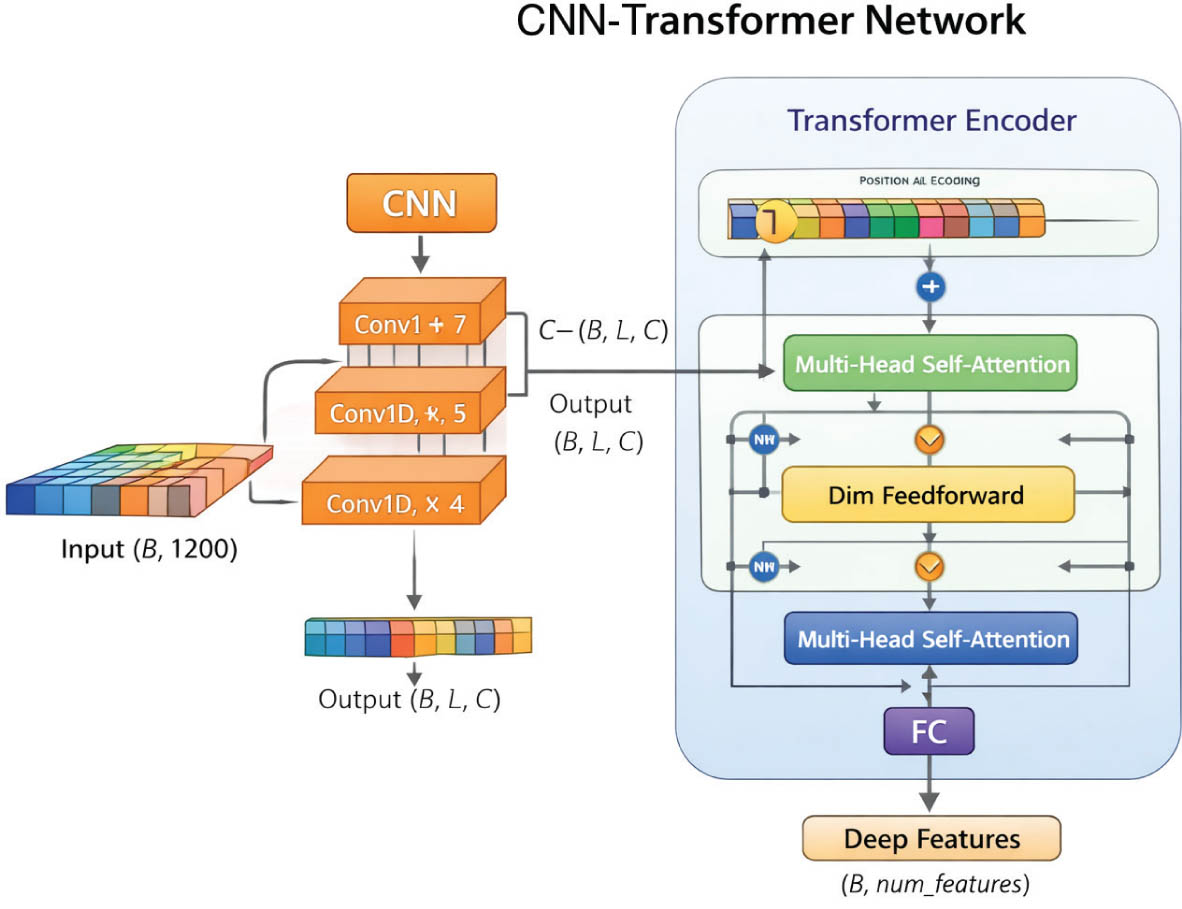
Figure 2:
Deep features extraction using CNN-transformer. CNNs, convolutional neural networks.
e. Convolutional feature learning
The CNN extracts local temporal features from signal segments. The convolution operation is defined by the following expression Eq. (2):
where wi represents convolution kernel weights and K denotes the kernel size. Multiple convolution layers progressively learn hierarchical features such as vibration impulses and oscillatory patterns.e.i. Positional encoding
Since transformer models do not inherently capture sequence order, positional encoding is incorporated to preserve temporal information. The encoded representation is expressed as:
where P represents the positional encoding matrix.e.ii. Transformer encoder
The transformer encoder utilizes self-attention mechanisms given by expression Eq. (4) to capture long-range dependencies in vibration signals. The attention mechanism is expressed as
Where Q denotes query vectors, K denotes key vectors, V denotes value vectors, and dk represents the dimensionality of the key vectors.
f. Frequency and time–frequency feature extraction
However, the method of frequency and time–frequency feature extraction enhances vibration signal visibility by understanding where the energy in the signal lies regarding the frequencies, and how these frequencies change over time. Often, characteristic frequency components resulting from defect sites, shaft rotation, or bearing geometry are expected to be generated when rotating mechanical faults occur. Analysis in the frequency domain allows us to look for fault-related peaks, which sometimes cannot be found by straightforward statistical features of the time domain. Thus, frequency features can be of particular benefit for periodic fault pattern detection and for specific defect types.
While statistical features mainly characterize the overall amplitude characteristics of a signal and the distribution of features, time–frequency methods examine non-stationary signal behavior where frequency components change over time due to evolving fault conditions. Methods such as spectrograms or wavelet transforms enable simultaneous analysis over both the time and frequency domains, thereby detecting transient signal/frequency impulses and focal defect signatures. Frequency and time– frequency features complement rich domain knowledge, which is essential as deep learning models automatically learn complex representations from raw signals; they also improve interpretability, robustness, and accuracy of the fault diagnosis system.
To complement deep representations, several spectral and time–frequency features are extracted.
f.i. Spectral kurtosis
Spectral kurtosis expressed using Eq. (5) evaluates impulsive characteristics in the frequency domain:
where f – Individual frequency component in the spectrum; represents the location of spectral energy within the signal, f – Mean (average) frequency of the power spectrum; acts as the reference point around which frequency deviations are measured, and P(f) – Power spectral density at frequency f; indicates the energy or power associated with each frequency component of the signal.Overall, this formulation of spectral kurtosis highlights frequency bands with abnormal energy concentration or impulsive behavior, which is highly useful for detecting early mechanical faults such as bearing defects or gear damage.
f.ii. Peak frequency
The dominant vibration frequency is determined by the following Eq. (6):
where arg max – Argument of the maximum operator; returns the frequency value at which the power spectrum reaches its maximum. Overall, this expression identifies the frequency component with the highest vibration energy, which is useful for detecting characteristic frequencies associated with faults, such as bearing defects, imbalance, or misalignment.f.iii. Total harmonic distortion
Total harmonic distortion quantifies harmonic energy within the signal and is given by Eq. (7) as:
where H1 – Amplitude of the fundamental harmonic (first harmonic); represents the primary vibration frequency of the system, Hn – Amplitude of the nth harmonic component in the frequency spectrum, and n – Harmonic order index (n = 2, 3, 4,... ) represents higher-order harmonics beyond the fundamental frequency.Overall, total harmonic distortion (THD) quantifies the amount of distortion caused by harmonic components in a vibration signal, which can indicate abnormal mechanical behavior such as misalignment, looseness, or bearing defects.
f.iv. Discrete wavelet transform
The signal is decomposed into multiple frequency bands using the discrete wavelet transform:
where cj,k – Wavelet coefficients indicate the contribution (energy or magnitude) of the signal at a specific scale j and position k, and ψj,k (t) – Wavelet basis function (scaled and shifted version of the mother wavelet); used to analyze localized signal characteristics. Wavelet decomposition effectively captures non-stationary characteristics of vibration signals.In our work, we used the Haar wavelet (db1) for discrete wavelet transform feature extraction. Such selection is based on bearing fault signals, which typically exhibit sudden and transient spikes due to impulsive mechanical impacts. To reflect this discontinuity, Haar wavelets, because they have the characteristic of a step-like basis function and remarkable time localization ability, work great.
While higher-order wavelets (e.g., Daubechies and Symlets) offer a higher level of smoothness and frequency resolution, they potentially suppress the sharp transients that are critical in fault characterization. In addition, they raise computational complexity without providing a substantial improvement in classification performance for the examined dataset. Initial experiments using db4 showed similar accuracy levels, which provided a rationale for the Haar wavelet as a computationally efficient alternative.
g. Feature fusion
To leverage complementary information from multiple domains, the extracted features are concatenated into a unified feature vector as shown in Figure 3 and expressed as:
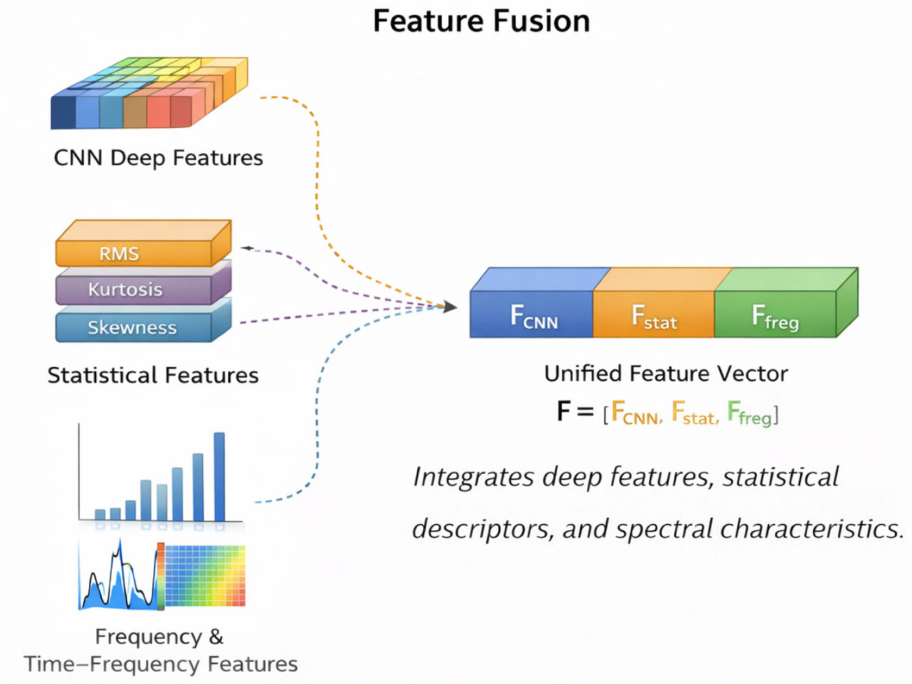
Figure 3:
The feature fusion integrating diverse features. CNNs, convolutional neural networks; RMS, root mean square.
This hybrid representation integrates deep features, statistical descriptors, and spectral characteristics. Figure 4 provides the distribution of various features to constitute the final feature vector.
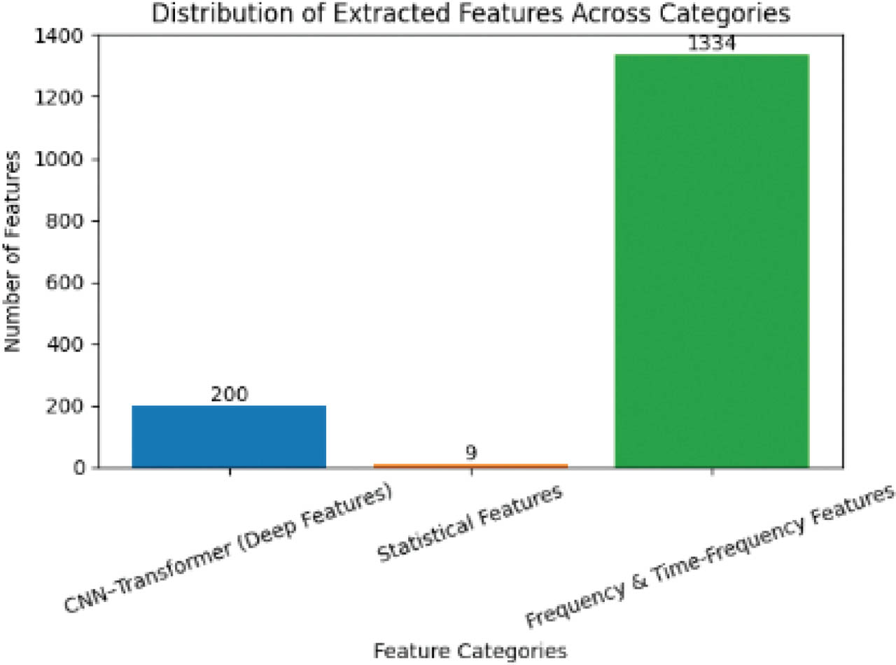
Figure 4:
Distribution of extracted features across different feature categories, illustrating the contribution of deep learning features, statistical descriptors, and frequency/time–frequency features in the fused feature representation. CNNs, convolutional neural networks.
Each representative sample shown in Figure 5 can be seen in the three-dimensional visualization, which allows us to visualize a sample distribution of all 10 bearing fault categories in the reduced feature space obtained through dimensionality reduction. This is a multilayer problem as each point represents an individual sample and multiple colors represent the fault classes.
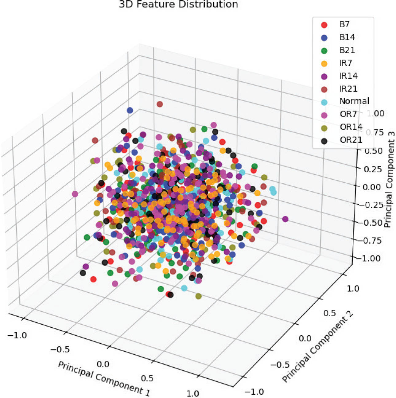
Figure 5:
3D visualization of the extracted hybrid feature space obtained using PCA dimensionality reduction, illustrating the separability of the 10 bearing fault categories.
h. Fault classification using a DNN
The final stage shown in Figure 6 employs a deep feedforward neural network for multi-class fault classification.
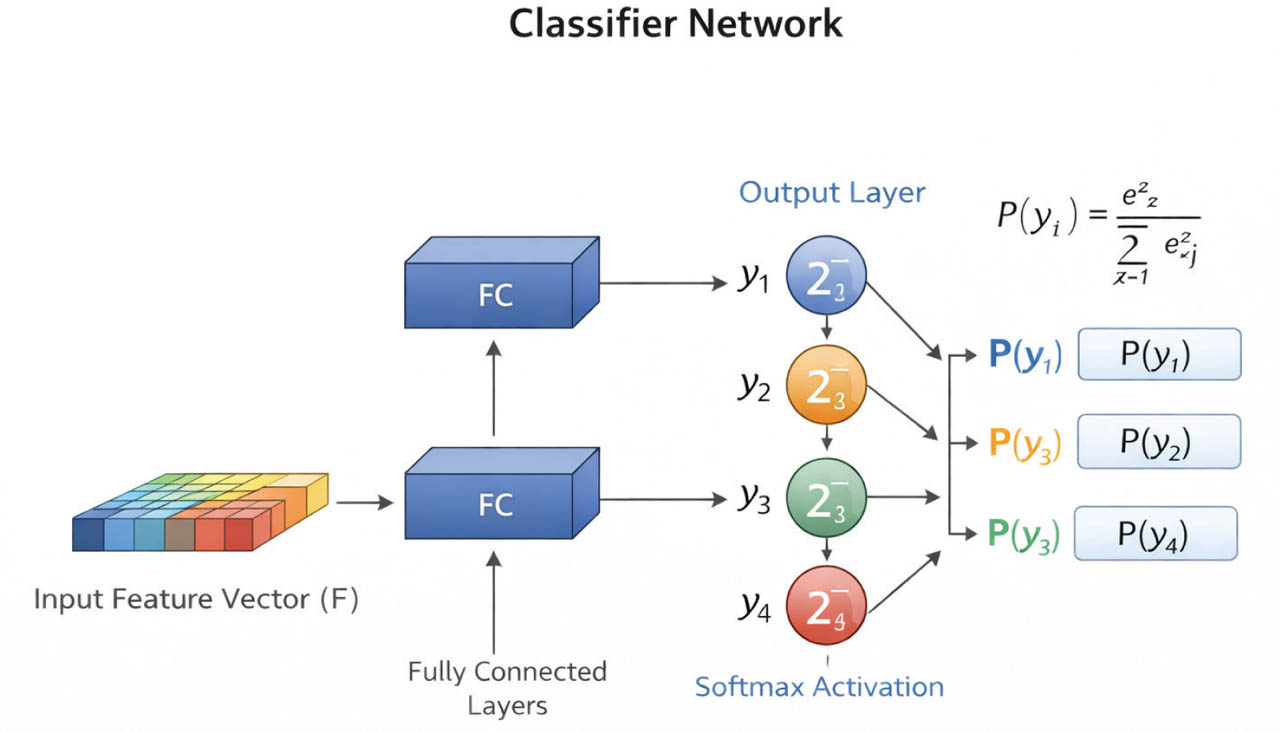
Figure 6:
The fault classifier network.
Each neuron computes
where W represents weights, b represents bias, and f (·) denotes the activation function.The ReLU activation function is used in hidden layers:
For multi-class classification, the output layer utilizes softmax activation, which is expressed using Eq. (11):
where C denotes the number of fault classes. Predicted probability of the input sample belonging to class i; represents the normalized output of the neural network. zi – Logit or raw output score of the neural network for the class i before activation. ezi – Exponential transformation of the logit value; ensures all outputs are positive and emphasizes larger scores.i. Model training and optimization
The model is trained using the categorical cross-entropy loss function expressed using Eq. (12):
where yi is the true label and is the predicted probability. The RMSprop optimizer is used to update network parameters by adaptively adjusting learning rates.The classification accuracy is first used to determine the fraction of correctly classified samples among all the ones tested. In addition, a confusion matrix is used to display a large number of correct and incorrect predictions for each fault category, to visualize it in detail. Precision and recall metrics are also computed to help determine how well the model is able to identify each individual fault class. For these metrics, the F1-score (which is defined as the harmonic mean of precision and recall) is used to evaluate any trade-off between those two measures. Taken together, the evaluation measures represent a comprehensive overview of the model's ability to classify varying bearing fault conditions for both accuracy and reliability.
The proposed method applies signal processing methods combined with deep learning models to leverage handcrafted and learned features. The CNN layers efficiently perceive local vibration patterns, and the transformer encoder encodes long-range temporal dependencies. The addition of spectral and wavelet information improves fault sensitivity. The hybrid methods of feature fusion, along with deep neural classification, enhance the diagnostic performance and robustness considerably, and make the framework applicable in practical industrial condition monitoring applications. The initial configuration parameters and hyperparameter settings used in the proposed fault diagnosis frame-work are listed in Table 2.
Table 2:
Initial configuration parameters and hyperparameter settings used in the proposed fault diagnosis framework, including signal segmentation parameters, CNN-transformer architecture settings, and classifier training configurations
| Parameter | Value used | Description |
|---|---|---|
| Sampling frequency | 48,000 Hz | Sampling rate used for vibration signal acquisition in the dataset |
| Segment length | 1,200 samples | Number of signal samples used in each segment |
| Number of segments per class | 318 | Total segments extracted from each bearing condition |
| Total classes | 10 | Number of bearing conditions (B7, B14, B21, IR7, IR14, IR21, Normal, OR7, OR14, OR21) |
| CNN input length | 1,200 | Length of the signal segment fed into the CNN |
| Transformer attention heads | 8 | Number of heads used in multi-head self-attention |
| Transformer layers | 2 | Number of stacked transformer encoder layers |
| Deep feature dimension | 200 | Output feature size from CNN-transformer feature extractor |
| Statistical features | 9 | Max, Min, Mean, Std, RMS, Skewness, Kurtosis, Crest Factor, Form Factor |
| Wavelet type | Haar | The mother wavelet used in the discrete wavelet transform |
| Wavelet decomposition level | 3 | Number of decomposition levels in DWT |
| Batch size | 32 | Number of samples processed per training batch |
| Training epochs | 400 | Total number of training iterations |
| Train-test split | 80%/20% | Dataset division for training and testing |
| Dropout rate (Layer 1) | 0.5 | Dropout applied after the first dense layer |
| Dropout rate (Layer 2) | 0.2 | Dropout applied after the second dense layer |
| Output layer neurons | 10 | Corresponds to the number of fault classes |
In the framework development work presented, RMSprop was adopted as the optimization algorithm of the CNN-transformer model to train the proposed CNN-transformer algorithm. RMSprop is especially applicable for non-stationary objectives and noisy gradient problems, as in vibration signal-based fault diagnosis tasks. Being that it trains using a moving average of squared gradients, its adaptive learning strategy provides a stabilization mechanism to update the updates based on highly fluctuating time-series data.
While Adam and AdamW are popular for transformer architectures, these are primarily built for large-scale deep learning problems, and they can introduce additional variance in smaller-scale industrial datasets. Adam and AdamW were evaluated in the same training settings as in the preliminary experiments. In the study, RMSprop showed similar or even superior convergence stability and test performance on the dataset analyzed. Accordingly, RMSprop is chosen as it offers a more robust and computationally efficient optimization algorithm for the hybrid architecture proposed here.
IV. Results and Discussion
To assess the convergence characteristics of the proposed hybrid fault diagnosis framework and its ability to generalize, it was examined for 400 epochs and 25 runs. Figure 7 shows the evolution in training and validation accuracy and loss curves. The accuracy curve shows a fast increase during the initial training phase, when the model quickly picks up discriminative representations from the hybrid feature space. During the first few epochs, a sudden rise in training accuracy is observed, which achieves a stable performance of around 99.9%, indicating proper feature learning and parameter optimization. The validation accuracy closely follows the training accuracy, which shows the high generalization property of the model and demonstrates minimal overfitting.
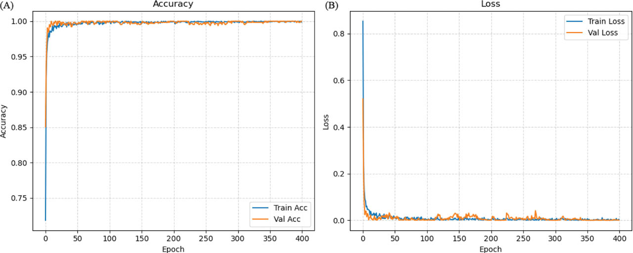
Figure 7:
Training performance of the proposed fault diagnosis model over 400 epochs, showing (A) training and validation accuracy curves and (B) training and validation loss curves, illustrating stable convergence and strong generalization capability.
Likewise, the loss curves shown in Figure 7B illustrate the optimization behavior of the network during training. The relatively small difference between training and validation loss results is evidence that our proposed model holds stable learning dynamics and avoids significant overfitting, and so is highly compatible with current techniques for performance. That the two curves also converge smoothly implies that the chosen optimization strategy and hyperparameters have been effectively used to guide the network toward a stable solution. The last summary of the training results after 400 epochs is: training accuracy: 99.88%, validation accuracy: 99.69%, training loss: 0.0040, and validation loss: 1.9435e-04. These data show that hybrid feature representation and CNN-transformer architecture effectively capture the discriminative characteristics of vibration signals for different bearing fault conditions.
For further investigation, the proposed framework's classification performance was evaluated on several performance metrics such as precision, recall, F1-score, and confusion matrix analysis. The model generates a total test accuracy of 99.98% (average over 20 runs), showing that the proposed approach can reliably identify different bearing fault conditions with high accuracy. It has been proven in the detailed classification report that almost all classes (except B21 and OR7) obtain a precision and recall of 1.00, indicating that learned feature representations are robust to prediction variation. The overall performance is exceptionally high at approximately 1.00 macro-average and weighted-average F1-scores.
Figure 8 shows the confusion matrix, which is used to understand the classification results of each fault category. This demonstrates that most predictions are concentrated along the primary diagonal, signifying that the classification of the corresponding fault conditions is correct. One diagonal element shows the number of true predictions for a class. The vast majority of fault classes display perfect classification performance without misclassified instances.
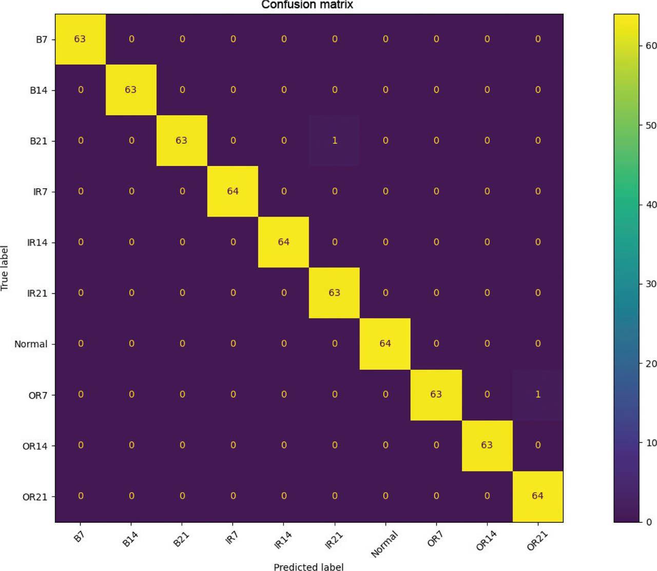
Figure 8:
Confusion matrix of the proposed CNN-transformer-based hybrid features fusion model for multi-class bearing fault diagnosis, showing the distribution of correctly and incorrectly classified samples across 10 fault categories. CNNs, convolutional neural networks.
The experiment results confirm that the proposed hybrid fault diagnosis framework is performing very well with high accuracy for the classification of the bearing fault dataset. Combining deep features that are extracted using a CNN-transformer architecture with descriptive statistics and frequency-domain descriptors, the model effectively captures both global signal patterns and localized transient characteristics in vibration data. These high-performance metrics and consistently strong evaluation metrics demonstrate how efficiently the proposed feature fusion approach is improving the discriminative power of the model. Furthermore, similar performance across all fault types demonstrates the robustness of the scheme, pointing to its suitability to establish reliable fault detection in practical RM condition monitoring applications.
a. Ablation studies
To test the efficacy of the transformer encoder, an ablation shown in Table 3 was conducted with a CNN-only baseline. The baseline used the same three convolutional layers as the proposed model but omitted the positional encoding and the transformer encoder. The output models had feature vectors of the same dimensionality and were used under the same training and testing conditions. The CNN-only model shown in Figure 9 was able to obtain the local fault-specific data from the vibration signals. Its receptive field was still constrained by convolution operations. By contrast, the transformer encoder allowed the temporally distant signal regions to interact directly via the self-attention mechanism, preserving long-range dependencies, which are hard to model by convolution alone.
Table 3:
Performance comparison between CNN-only and CNN + transformer-based feature extraction
| Model | Accuracy (%) | Precision (%) | Recall (%) | F1-score (%) |
|---|---|---|---|---|
| CNN-only | 96.12 | 95.84 | 95.67 | 95.80 |
| CNN + transformer | 99.98 | 99.68 | 99.68 | 99.80 |
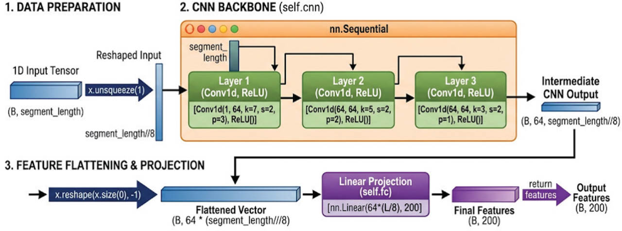
Figure 9:
Architecture of the CNN-only feature extractor module, illustrating the transformation of a 1D sequence into a fixed-size feature vector through successive convolutional downsampling and linear projection. 1D, one-dimensional; CNNs, convolutional neural networks.
The CNN-only feature extractor network consists of a 1D input tensor of shape (B, segment_length,) and first unsqueezes this to create a channel dimension, obtaining a shape of (B,1, segment_length). Then, this rewritten input needs to be fed into a convolutional backbone with three consecutive Conv1d layers layered over each other with ReLU activation. The kernel size for the first layer is 7 (s = 2, p = 3), for the second layer is 5 (s = 2, p = 2), and the final layer is 3 (s = 2, p = 1). Since every one of these three layers uses a stride of 2, the spatial length of the sequence is reduced (systematically) at every step, generating an output of shape (B,64, segment_length / /8) whose channel dimension grows to 64. This multi-channel feature map is subsequently flattened to a 1D B × (64 × (segment_length / /8)) vector by the reshaping operation. A fully connected linear layer finally reduces this flattened vector to a more compact representation in a fixed size of 200 features; hence, the final tensor of shape (B,200) is then produced.
Table 3 demonstrates that the proposed CNN-transformer model achieves superior performance compared with the CNN-only baseline, confirming the effectiveness of incorporating the transformer encoder for vibration-based fault diagnosis.
The comparative analysis of wavelet functions shown in Table 4 revealed that the Haar wavelet (db1) achieves the best performance with an accuracy of 99.98% and the lowest training time among all tested configurations. This superior performance can directly be attributed to its ability to capture abrupt transient changes in vibration signals, which indicate high fault conditions. This performance is in stark contrast with higher-order wavelets such as db4 and sym4, which achieved accuracies of 98.3% and 98.1%, respectively, although they had better frequency localization capabilities. But their smoothness tends to suppress the sharp discontinuities in the signal, which are vital for accurate fault discrimination, and it also increases the computational complexity, hence the training time.
Table 4:
Performance comparison of different wavelet functions for feature extraction in bearing fault diagnosis, showing classification accuracy and computational efficiency
| Wavelet | Accuracy (%) | Training Time | Interpretation |
|---|---|---|---|
| Haar (db1) | 99.98 | Low | Best performance, fastest computation |
| db4 | 98.3 | Medium | Good frequency localization, but lower accuracy |
| sym4 | 98.1 | Medium | Smooth wavelet, but slightly less effective here |
The obtained results show that the Haar wavelet (db1) has a trade-off between high efficiency and discriminative features for fault diagnosis. Because it captures the sudden perturbations, such as instantaneous transient events in vibration signals efficiently, it achieves better classification performance. On the other hand, high-order wavelets like db4 and sym4 provide better smoothness and frequency localization, but they often hide sharp perturbations, and therefore, their classification accuracy suffers from this.
Likewise, considering optimization algorithms depicted in Table 5, the performance of RMSprop is proven considerably better than the effectiveness of Adam and AdamW, achieving 99.98% accuracy with a very short convergence time, with stable high data. The adaptive learning strategy of RMSprop, using a moving average of squared updates to normalize gradients can significantly help it to deal with noisy and non-stationary vibration signals. However, Adam gives faster convergence but less stable updates, meaning less stable update time and therefore worse accuracy (98.1%); AdamW, with even better regularization in terms of decoupled weight decay, achieves 98.2% accuracy and medium convergence speed. Taken together, RMSprop proves to have better generalization and stability performance for the proposed CNN-transformer framework than Adam and AdamW, which results in the best performance as the most promising optimizer for this application.
Table 5:
Comparative evaluation of optimization algorithms for training the proposed CNN-transformer model in terms of accuracy, convergence speed, and stability
| Optimizer | Accuracy | Convergence speed | Stability | Interpretation |
|---|---|---|---|---|
| RMSprop | 99.98% | Fast | High | Best overall performance |
| Adam | 98.1% | Fast | Medium | Good, but less stable here |
| AdamW | 98.2% | Medium | Medium | Regularized but slower convergence |
The output in Table 6 showed that each feature category is informative in terms of discriminative information, and the fused feature representation achieved the best result across all evaluation metrics. It is shown that the convergence of heterogeneous groups of features yields higher classification performance than individual feature sets or partial combinations. In this context, deep features represent CNN hierarchical representations, statistical features reveal distributional characteristics of the signal, and frequency-domain features represent spectral properties. These representations complement each other, providing a more discriminative mechanism, so the ability to classify in that manner is better with a greater classification performance when all feature types are combined.
Table 6:
Ablation study evaluating the contribution of individual and combined feature sets (deep, statistical, and frequency-domain features) on classification performance using accuracy, precision, recall, and F1-score
| Feature Type | Accuracy (%) | Precision (%) | Recall (%) | F1-score (%) |
|---|---|---|---|---|
| Deep features (CNN only) | 94.23 | 94.68 | 93.54 | 94.10 |
| Statistical features only | 91.66 | 90.28 | 89.57 | 89.97 |
| Frequency features only | 93.66 | 95.89 | 95.89 | 95.89 |
| Deep + statistical | 96.22 | 97.0 | 96.98 | 97.03 |
| Deep + frequency | 97.10 | 96.30 | 96.30 | 96.30 |
| Statistical + frequency | 95.00 | 97.12 | 95.55 | 96.12 |
| All fused (proposed) | 99.98 | 99.68 | 99.68 | 99.80 |
b. Comparative performance
Table 7 indicates the comparative analysis from that perspective, in which the proposed fault diagnosis framework is evaluated against some recent state-of-the-art methods developed specifically for bearing fault classification using the CWRU dataset. The results confirm that deep learning–based methods have shown reliably better diagnostic performance in recent years. For instance, Yoo et al. [20] suggested a lightweight deep learning model with ResNet-50 architecture and reached an accuracy of 99.97%, indicating the impact of compact CNN architectures for vibration-based fault diagnosis. Similarly, Mohiuddin et al. [21] utilized a modified version of the AlexNet model to achieve an accuracy of 98.30%, achieved a precision of 98.41% and a perfect recall of 100%, demonstrating that the detection of the fault classes was robust.
Table 7:
Comparative performance analysis of the proposed bearing fault diagnosis framework with recent state-of-the-art methods on the CWRU dataset
| Reference | Model | Accuracy | Precision | Recall | F1-score |
|---|---|---|---|---|---|
| Yoo et al. [20] | Resnet50 (Lite CNN) | 99.97 | - | - | - |
| Mohiuddin et al. [21] | Modified AlexNet | 98.30 | 98.41 | 100 | 99.20 |
| Zhang et al. [22] | Convolutional spiking neural network | 99.83 | - | - | - |
| Lee et al. [23] | XGBoost + PSO | 99.10 | 99.3 | 99.2 | 99.1 |
| Hatipoglu et al. [24] | LSTM-Attention and LASSO | 98.50 | - | - | 98.742 |
| Khan et al. [25] | RNN-XGBoostNet | 99.57 | 99.54 | 99.21 | 99.37 |
| Proposed | FaultFormer-Net | 99.98 | 99.68 | 99.68 | 99.80 |
A different high-grade approach is introduced by Zhang et al. [22], who proposed a convolutional spiking neural network that extracts features from the spatial–temporal dataset and achieves a 99.83% classification accuracy. Hybrid approaches have demonstrated impressive performance as well. For instance, Lee et al. [23] applied particle swarm optimization in the context of XGBoost to improve accuracy, obtaining a 99.10%, while Hatipoglu et al. [24] merged long short-term memory (LSTM) with attention mechanisms and LASSO-based feature selection to achieve an F1-score of 98.742. More recently, Khan et al. [25] proposed an RNN-XGBoostNet architecture with 99.57% accuracy with balanced precision, recall, and F1-score values.
Compared with these extant strategies, the proposed hybrid framework achieves 99.98% accuracy (mean over 20 runs), 99.68% precision, 99.68% recall, and 99.80% F1-score, indicating superior classification. This is attributed to the fact that it combines deep CNN-transformer features, and statistical and frequency domain descriptors, which means the new model can model global patterns as well as localized transient features of vibration signals. This comprehensive feature fusion strategy enhances the discriminative capacity of the classifier such that all 10 fault categories are consistently identified. Thus, the result shows a competitive and cutting-edge approach for intelligent fault prediction in a bearing fault diagnosis system and opens up avenues for future applications such as reliable commercial monitoring of industrial conditions.
V. Conclusion
Using a multi-domain feature fusion approach, the study proves that the FaultFormer-Net framework is more effective for intelligent fault diagnosis in detecting and repairing the mechanical failure of a bearing. This hybrid strategy seamlessly merges statistical descriptors' physical interpretability and deep learning's ability to represent them at a high level, which can bypass the difficulties involved in working with individual feature sets. The experimental results on the CWRU dataset provide the results for the model performance; it attains an appropriate performance in both the training accuracy of ~ 99.9% and the test accuracy of ~ 99.9% in all 10 fault categories. The close fit between training and validation curves, as well as smooth convergence, demonstrates a good generalization capability and low overfitting for different motor loading scenarios. This robustness is probably due to the integration of CNN-based local feature learning with Transformer-based long-range dependency capture, and additionally, the inclusion of spectral and wavelet data.
Ablation studies verified that the structure of the proposed framework will perform optimally when architecture, preprocessing, optimization, and feature fusion elements work symbiotically together. The Transformer encoder, when incorporated with the CNN backbone, improves fault-detection accuracy by taking account of long-range temporal dependencies, solving the receptive field imperfections associated with pure convolution. These architectural rigors are supported by the computationally efficient Haar (db1) wavelet, which keeps important, sharp transient perturbations that would be smoothed out by higher-order wavelets. Additionally, the RMSprop optimizer exhibits better stability and convergence over noisy, non-stationary vibration data than its Adam-based counterparts for the detection task. In the end, the heterogeneous deep, statistical, and frequency-domain features provide for a complete, multi-view signal representation, which can achieve an almost perfect classification accuracy (99.98%) and an F1-score (99.80%) that supports the soundness of the overall proposed framework for bearing fault diagnosis.
Lastly, the proposed framework is very accurate and reliable and could be put to work in industrial condition monitoring systems for commercial applications for early identification and classification of mechanical failures.
Notes
[8] Contributed by Author Contributions
Smita Bhuyarkar conceptualized the study, designed the proposed FaultFormer framework, performed methodology development, software implementation, data analysis, and experimental validation, and prepared the original draft of the manuscript, including visualization of results. Nilesh Deshmukh contributed to research supervision, methodological validation, and guided refining the technical approach, as well as reviewing and editing the manuscript. Narendra P. Giradkar assisted in experimental design, interpretation of results, and contributed to reviewing and improving the manuscript. All authors read and approved the final version of the manuscript.