
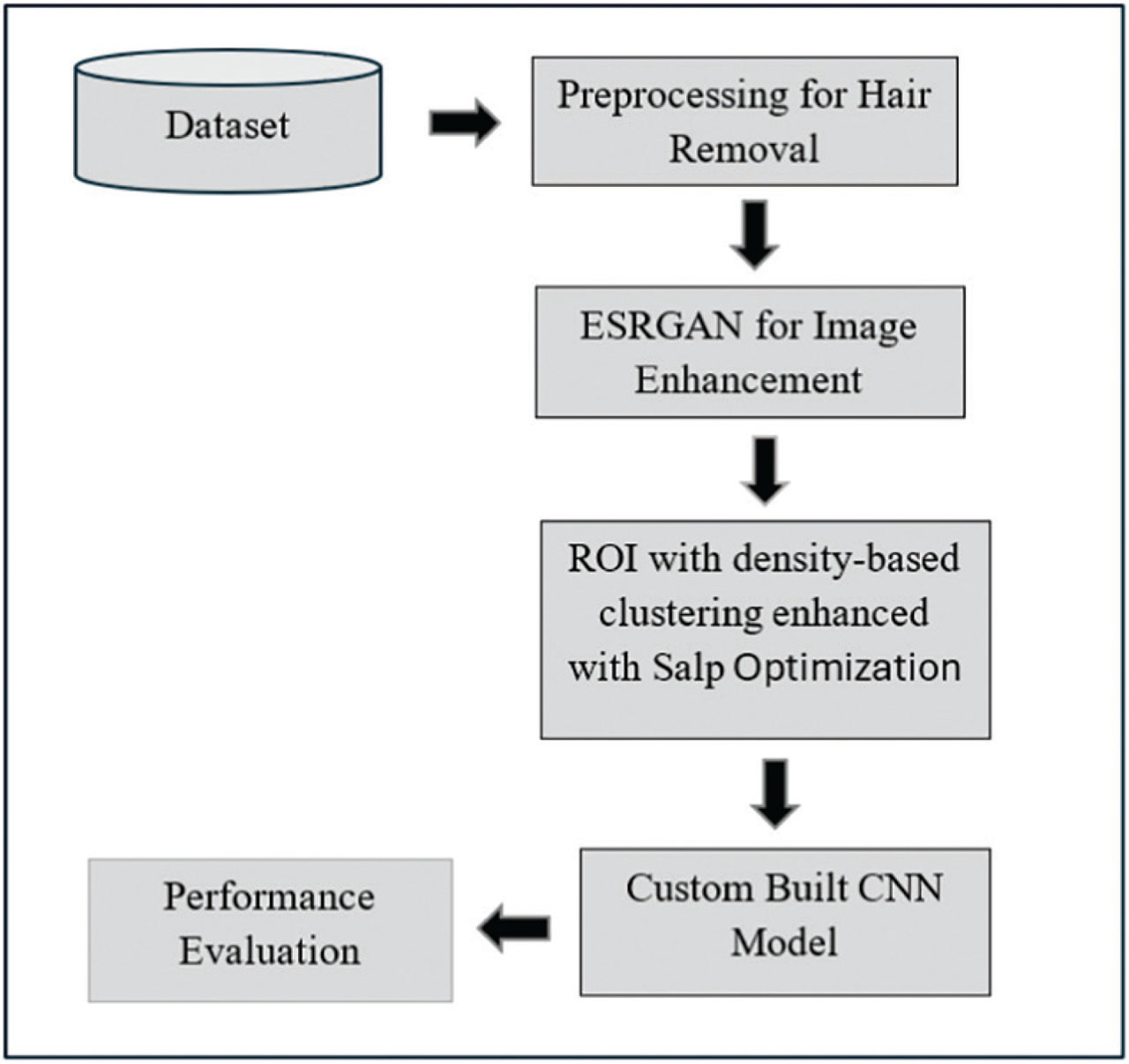
Figure 1:
Block diagram of proposed framework. ESRGAN, Enhanced super generative adversarial network.
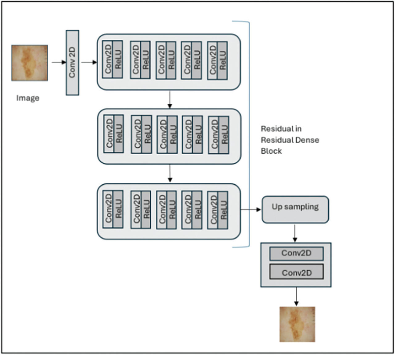
Figure 2:
Architecture of ESRGAN. ESRGAN, enhanced super generative adversarial network.
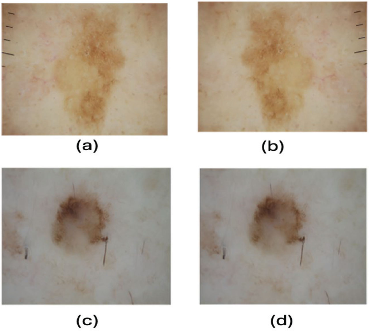
Figure 3:
(A) and (C) Original melanoma images and (B) and (D) the ESRGAN output images. ESRGAN, enhanced super generative adversarial network.
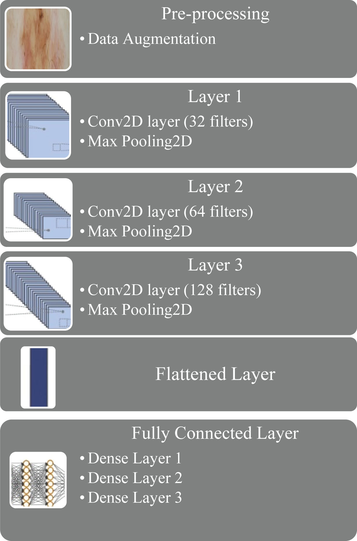
Figure 4:
Architecture of 3-layer CNN model.
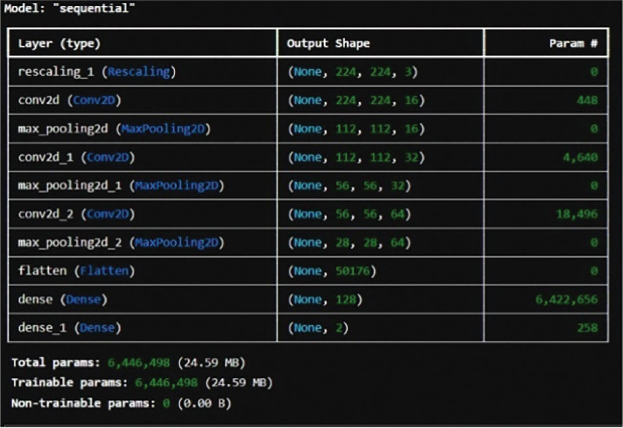
Figure 5:
Model summary for melanoma diagnosis.
Table 1:
Experimental results of the model proposed for melanoma image diagnosis
| Classifiers | Precision (%) | Recall (%) | F1-score (%) | Accuracy (%) |
|---|---|---|---|---|
| CNN model | 74.3 | 78.5 | 75.7 | 76.4 |
| CNN model with augmentation | 87 | 91.2 | 89.5 | 89 |
| ESRGAN + CNN | 92.9 | 91.6 | 92.3 | 92.2 |
| DBCESp + CNN | 90.4 | 91.2 | 91.0 | 91.0 |
| ESRGAN + DBCESp + CNN | 94.6 | 94.3 | 94.5 | 94.5 |
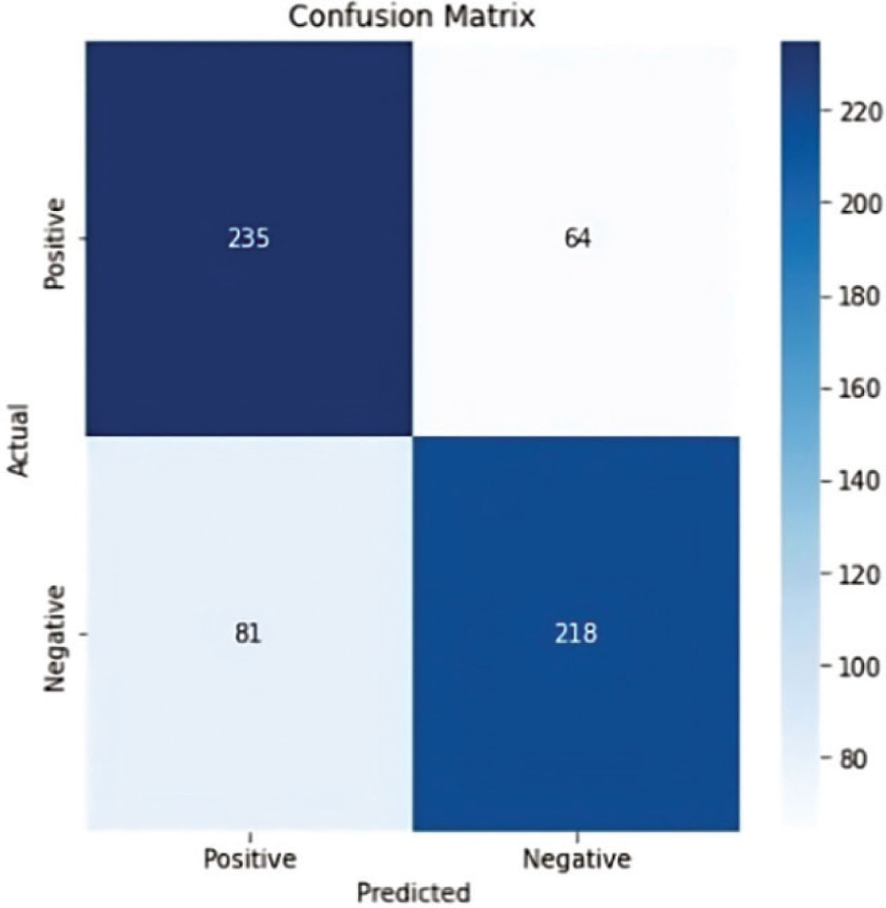
Figure 6:
Confusion matrix for simple three-layer CNN model without augmentation.
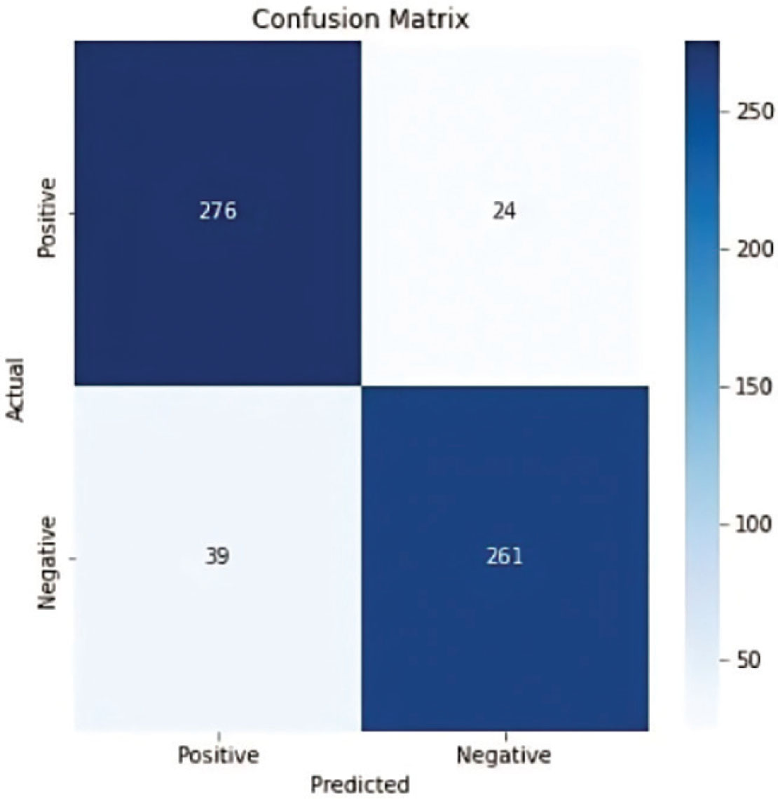
Figure 7:
Confusion matrix for CNN model with augmentation.
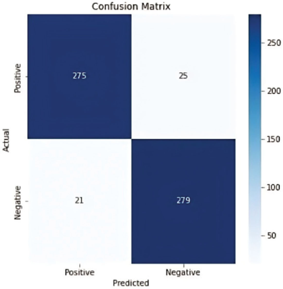
Figure 8:
Confusion matrix for model with CNN and ESRGAN. ESRGAN, enhanced super generative adversarial network.
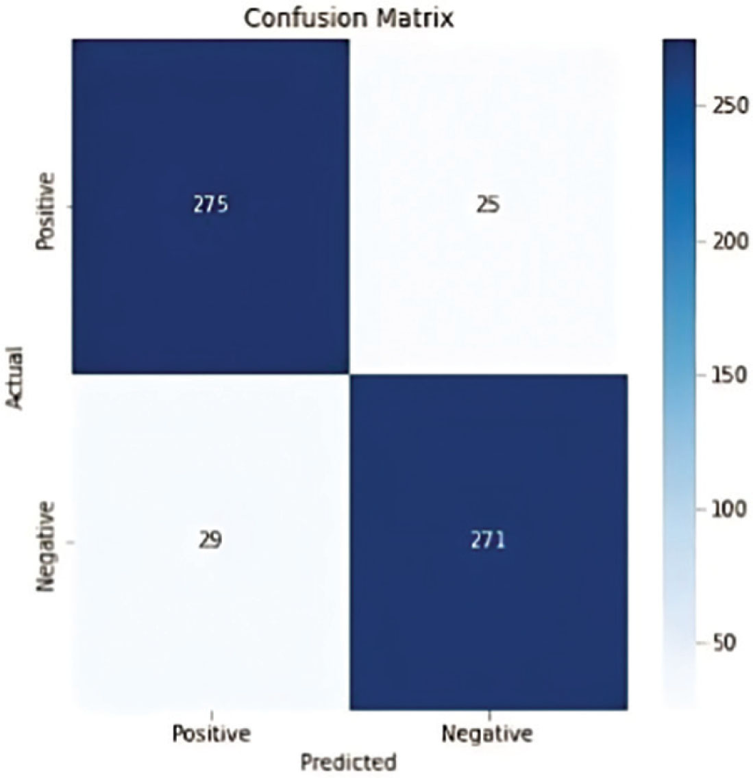
Figure 9:
Confusion matrix for model with CNN and DBCESp algorithm.
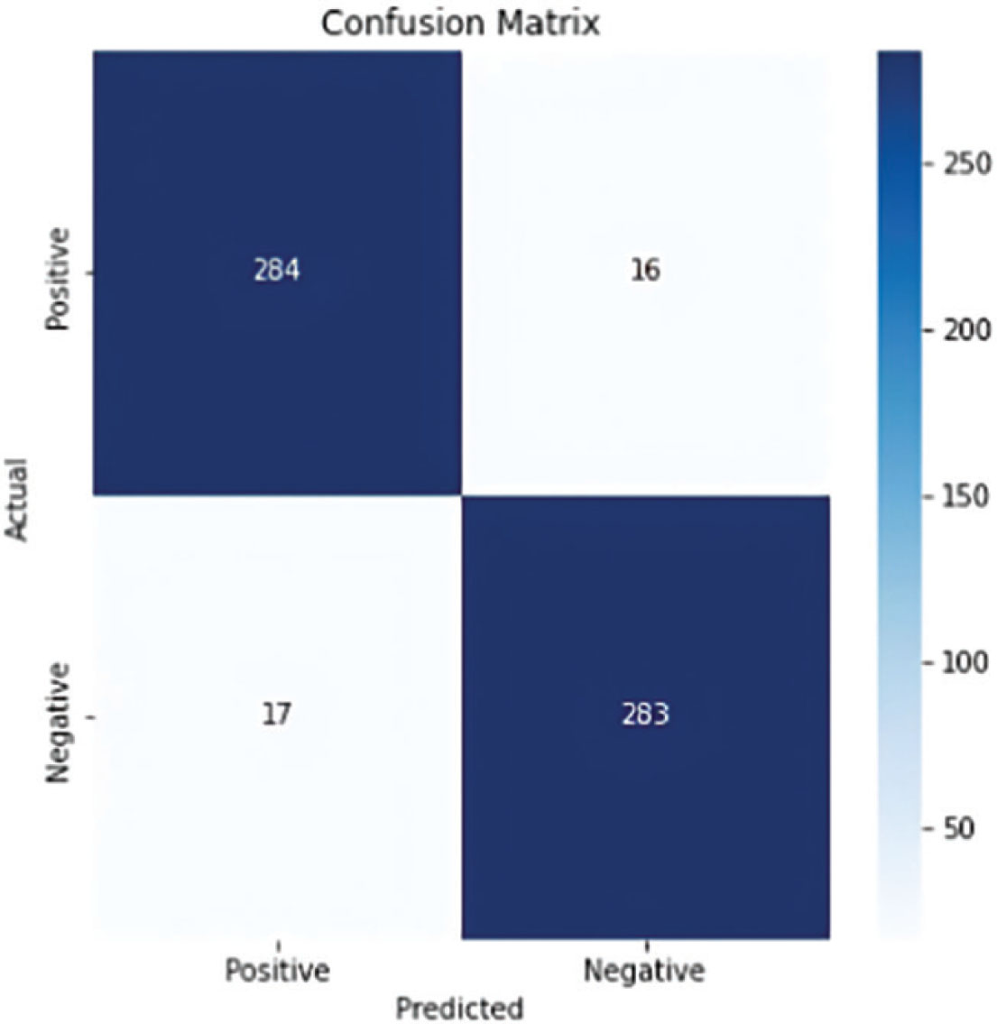
Figure 10:
Confusion matrix for melanoma diagnosis with proposed ESRGAN-DBCESp-CNN model. ESRGAN, enhanced super generative adversarial network.
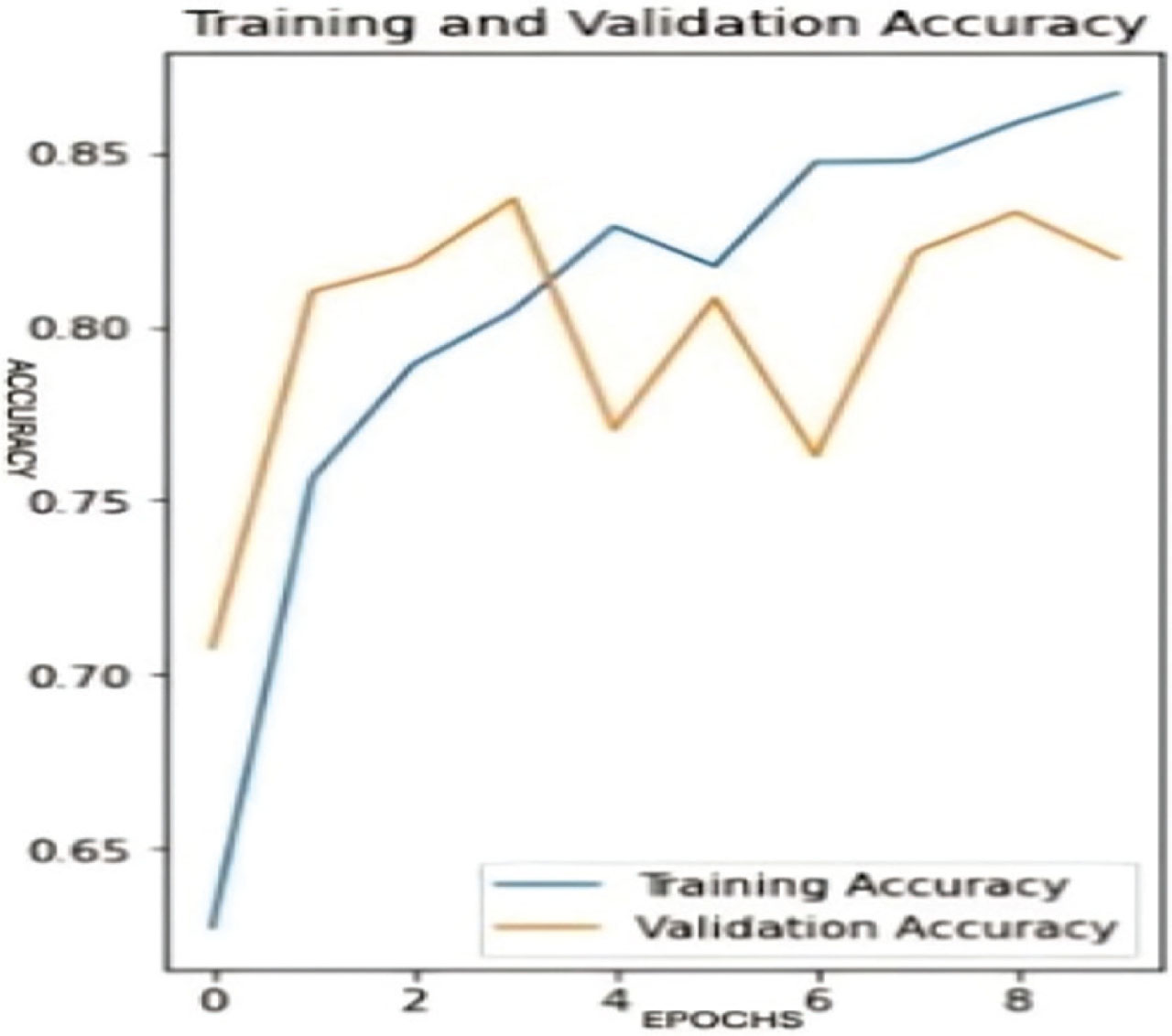
Figure 11:
Training and validation accuracy graph per Epochs for the simple CNN model.
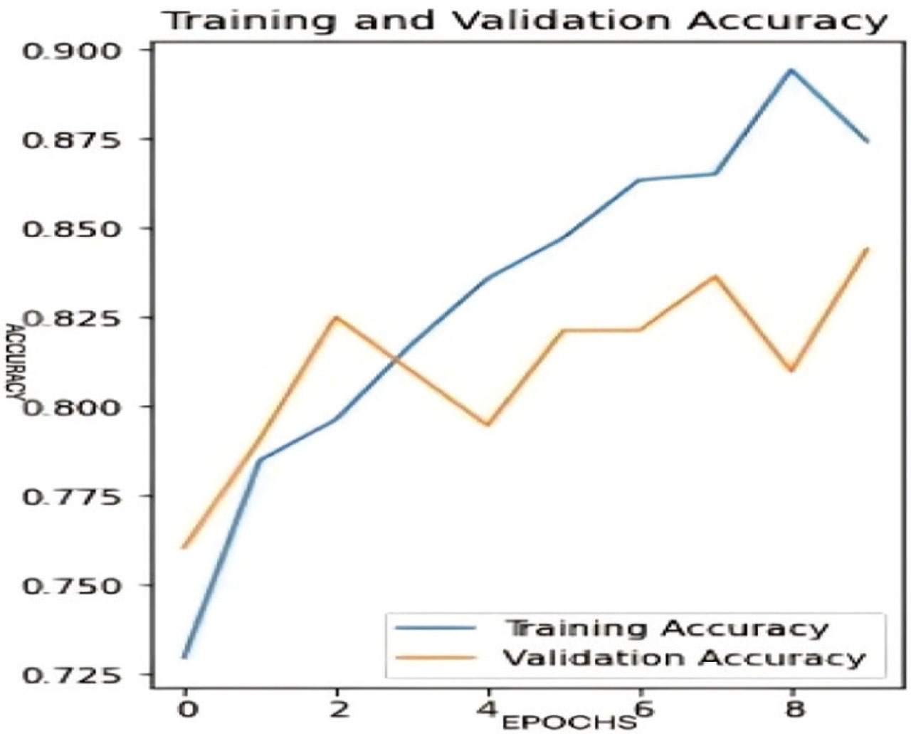
Figure 12:
Training and validation accuracy graph per epochs for the CNN model with ESRGAN. ESRGAN, enhanced super generative adversarial network.
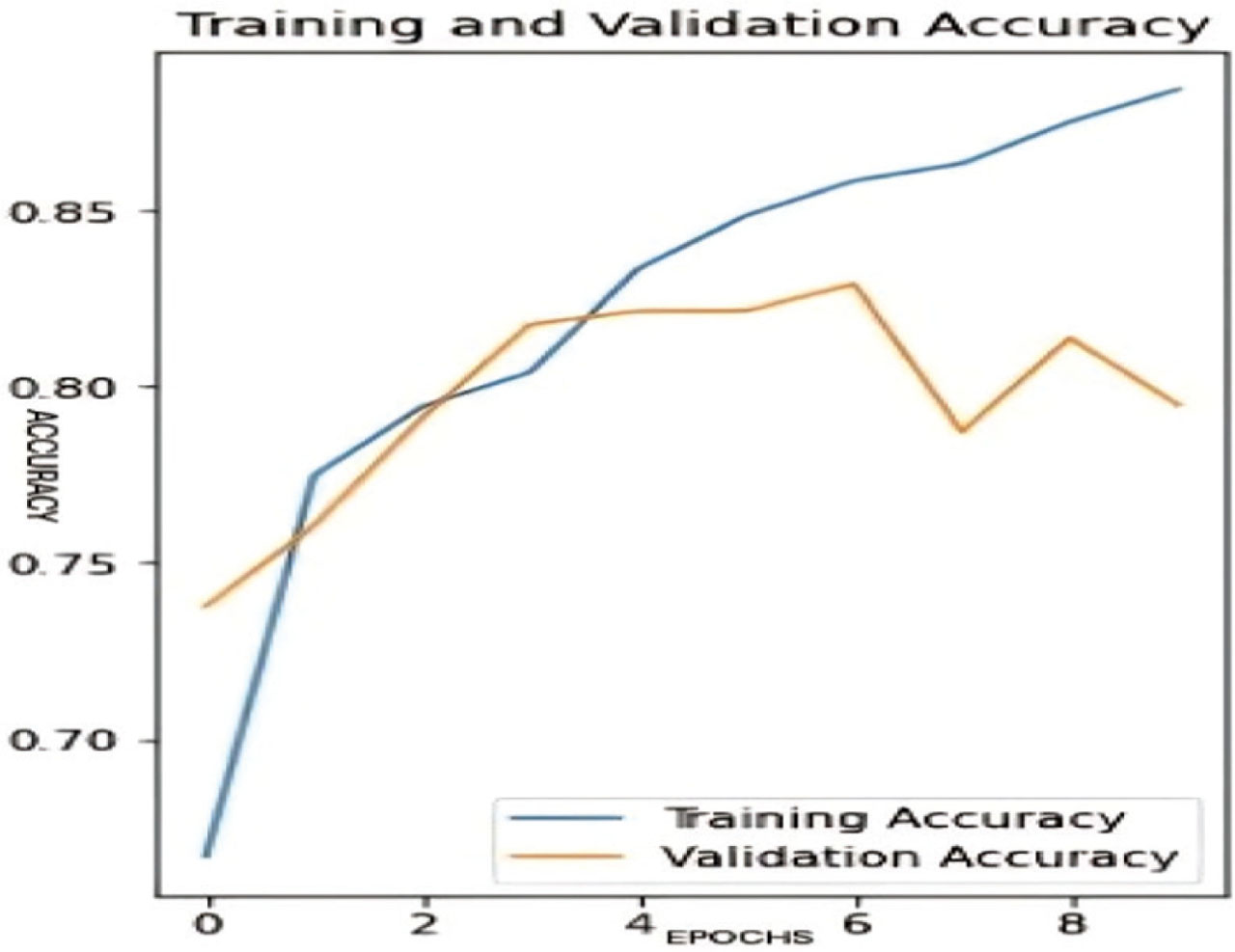
Figure 13:
Training and validation accuracy graph for ESRGAN-DBCESp-CNN framework. ESRGAN, enhanced super generative adversarial network.
Table 2:
Time complexity of DBCESp algorithm
| Steps | Complexity |
|---|---|
| Neighborhood search | O(nlog n) |
| Cluster formation | O(n) |
| Salp optimization - evaluating fitness | O(p.n) |
| Update Salp position and evaluate fitness of new solution with I iterations | O(I. p.n) |
| Total complexity | O(nlog n) + O(I. p.n) |
Table 3:
Time complexity of fuzzy C-means clustering algorithm
| Steps | Complexity |
|---|---|
| Initialization of membership matrix (m, n) | O(mn) |
| Compute cluster membership for each data point | O(m.n.d) |
| Cluster center updations | O(m.n.d) |
| Stop criteria | O(m.n) |
| Salp optimization algorithm | O(I. p.c) |
| Total complexity | O(m.n.d) + O(I. p.c) |
Table 4:
Performance evaluation of the four-layer CNN models
| Classifiers | Precision | Recall | F1-score | Accuracy |
|---|---|---|---|---|
| Four-layer CNN | 80.9% | 79.5% | 80.2% | 80.43% |
| Four-layer CNN model with BN and dropouts | 88.1% | 68.8% | 74.7% | 78.0% |
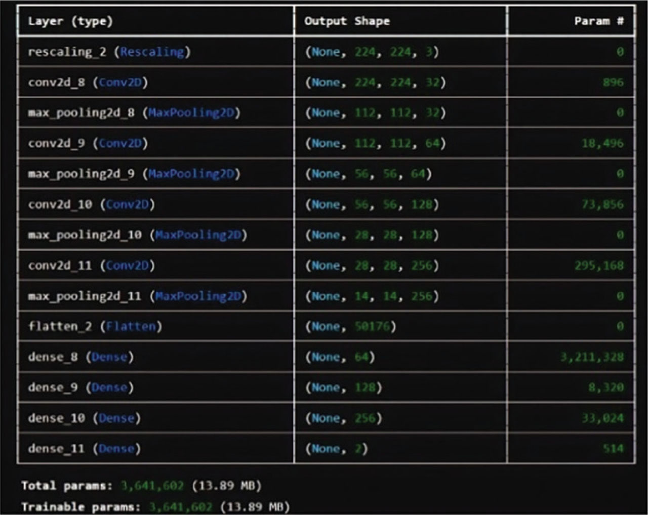
Figure 14:
Summary of four-layer CNN model without BN and dropouts. BN, batch normalization.
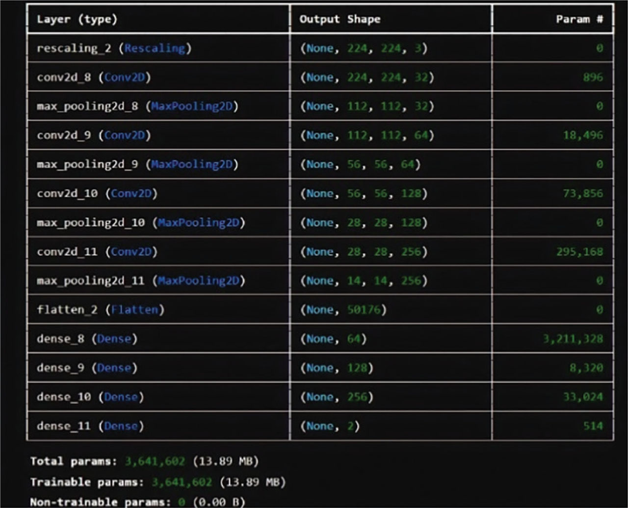
Figure 15:
Summary of four-layer CNN model with BN and dropouts. BN, batch normalization.
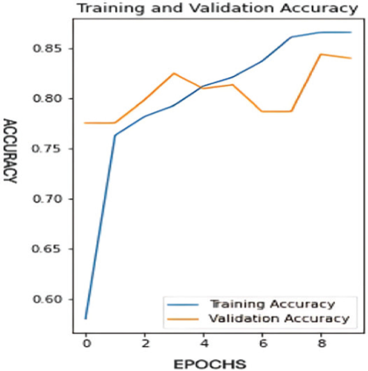
Figure 16:
Training and validation accuracy graph for four-layer CNN model without BN and dropout layers. BN, batch normalization.
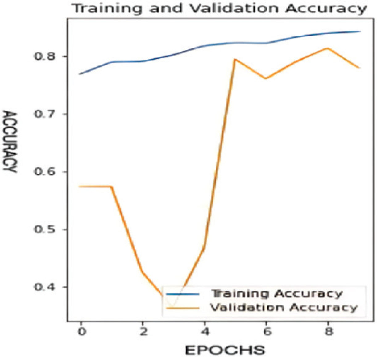
Figure 17:
Training and validation accuracy graph for four-layer CNN model with BN and dropout layers. BN, batch normalization.
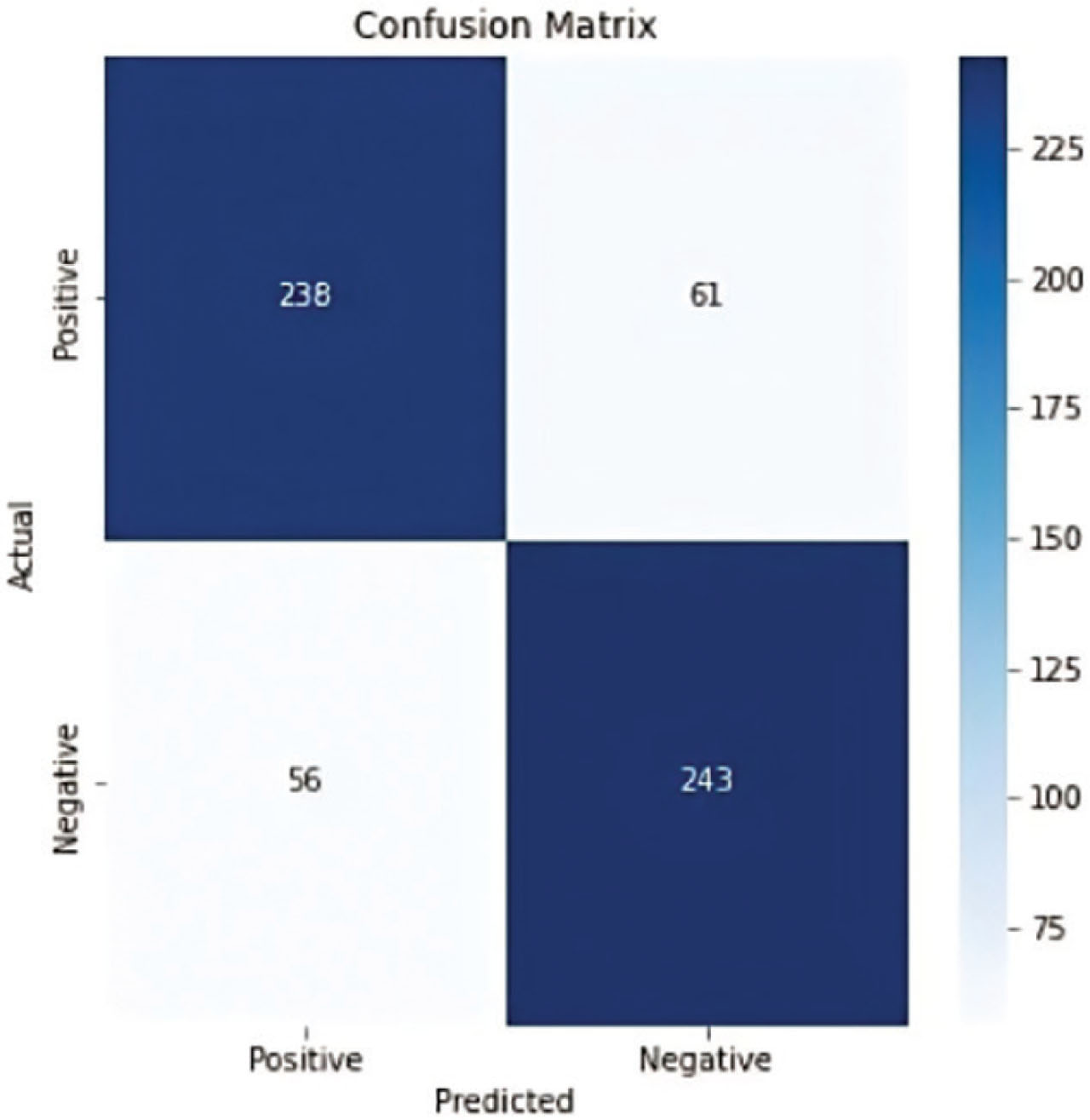
Figure 18:
Confusion matrix for CNN model without BN and dropout layers. BN, batch normalization.
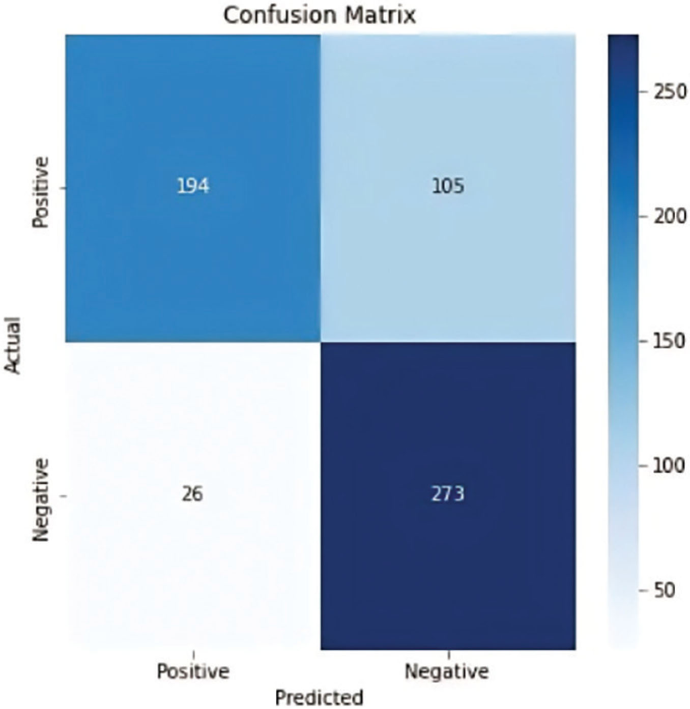
Figure 19:
Confusion matrix for CNN model with BN and dropout layers. BN, batch normalization.
Table 5:
Feature set extracted from the melanoma images
| Features | Feature set |
|---|---|
| Brightness Features | Luminance for LAB and YCBCR |
| HSV features | Hue, saturation, and value |
| Shape features | Area, perimeter, circularity, eccentricity, convex area, solidity, equivalent diameter |
| Texture features | Contrast, correlation, energy, homogeneity |
| Spatial features | Contour detection |
Table 6:
Experimental results of comparative study
| Classifiers | Precision | Recall rate | F1-score | Accuracy | |||
|---|---|---|---|---|---|---|---|
| B | M | B | M | B | M | ||
| SVM | 64 | 76 | 90 | 40 | 75 | 52 | 67 |
| LR | 64 | 73 | 88 | 40 | 74 | 52 | 66 |
| Desc tree | 78 | 74 | 78 | 74 | 78 | 74 | 76 |
| AdaBoost | 82 | 78 | 81 | 79 | 82 | 79 | 81 |
| Gradient boost | 83 | 77 | 81 | 81 | 83 | 80 | 81 |
| Random forest | 86 | 82 | 85 | 84 | 86 | 83 | 84 |
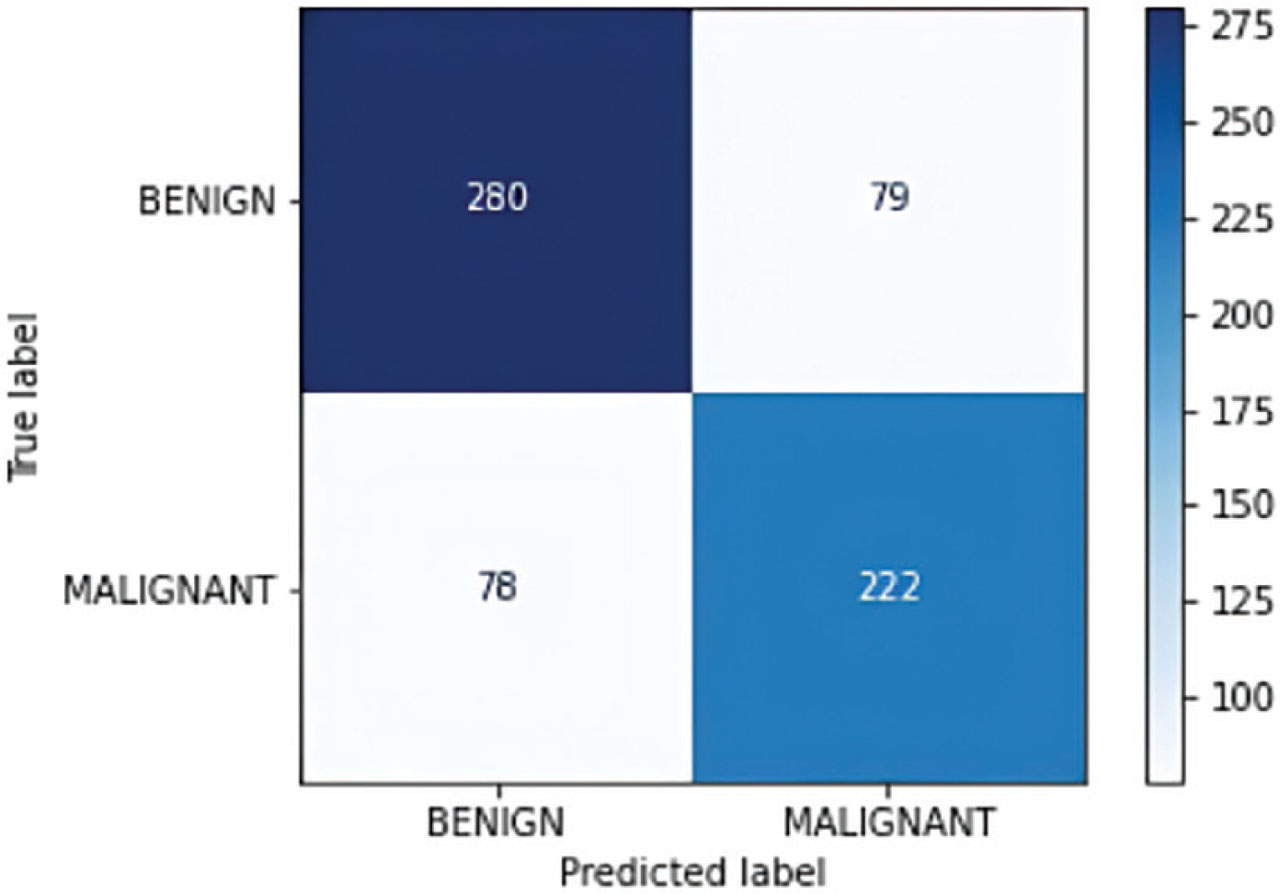
Figure 20:
Confusion matrix for SVM classifier.
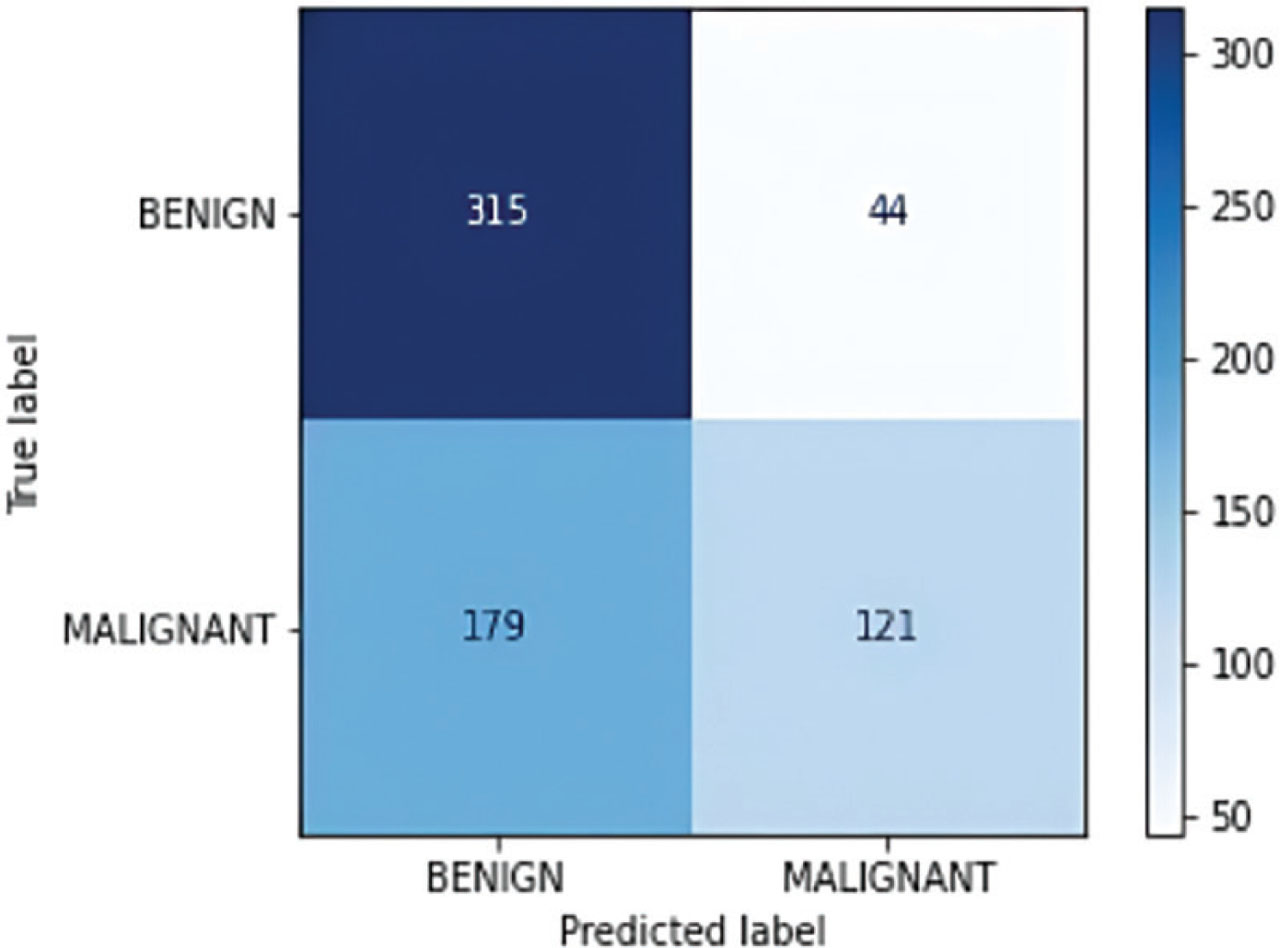
Figure 21:
Confusion matrix for logistic regression as classifier.
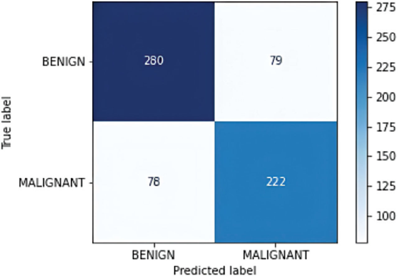
Figure 22:
Confusion matrix for decision tree as classifier.
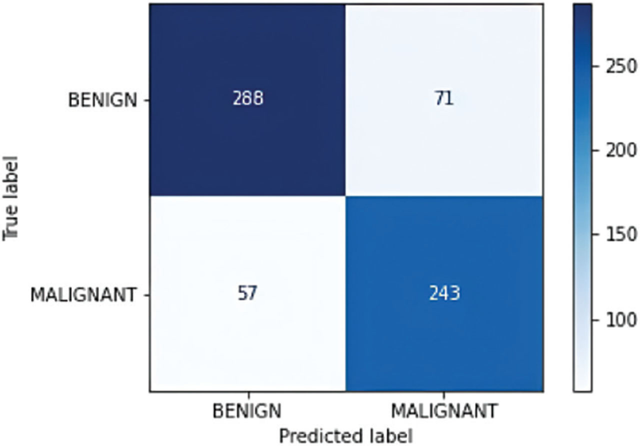
Figure 23:
Confusion matrix for AdaBoost as classifier.
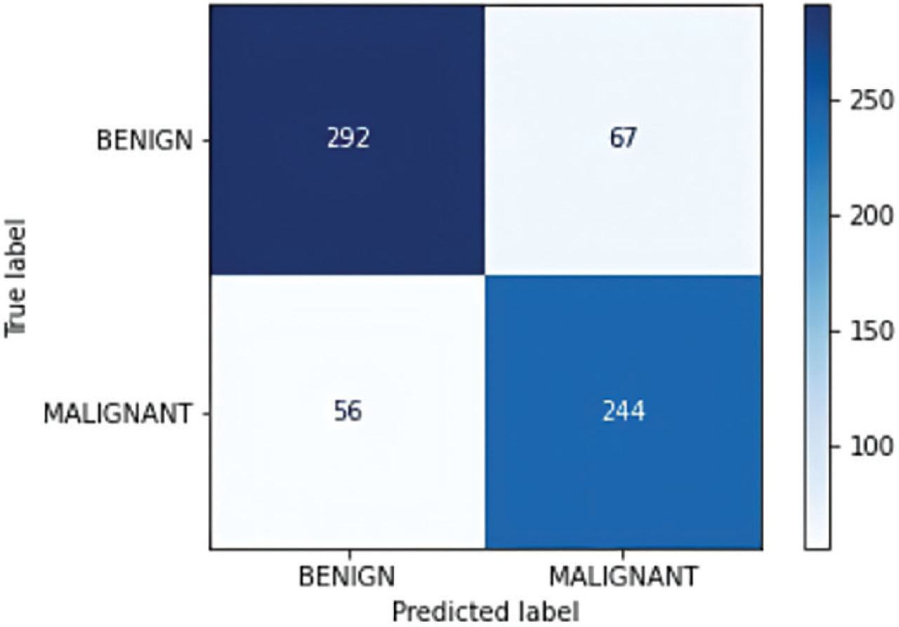
Figure 24:
Confusion matrix for gradient boosting as classifier.
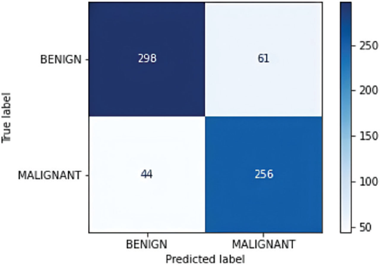
Figure 25:
Confusion matrix for random forest as classifier.
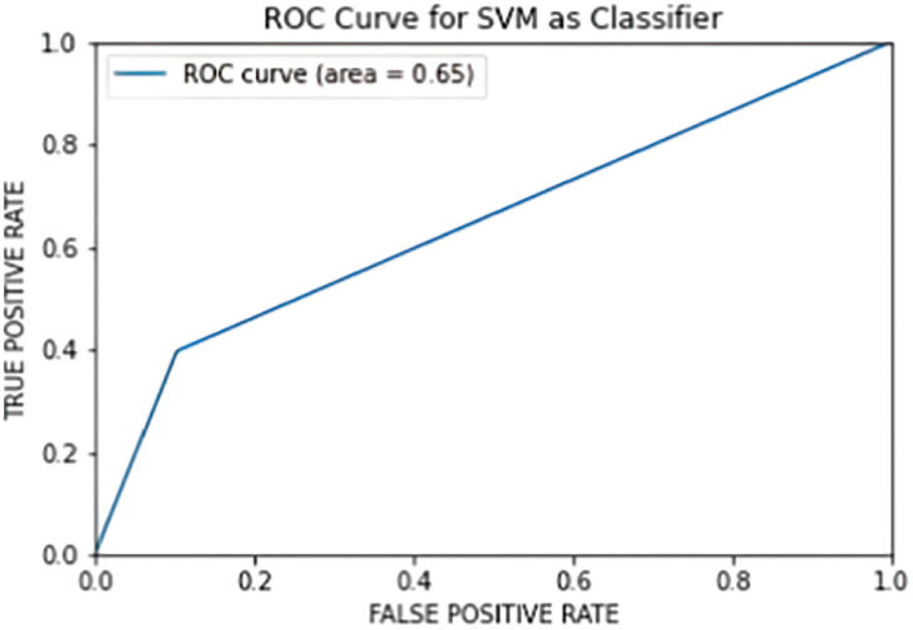
Figure 26:
ROC curve for SVM as classifier.
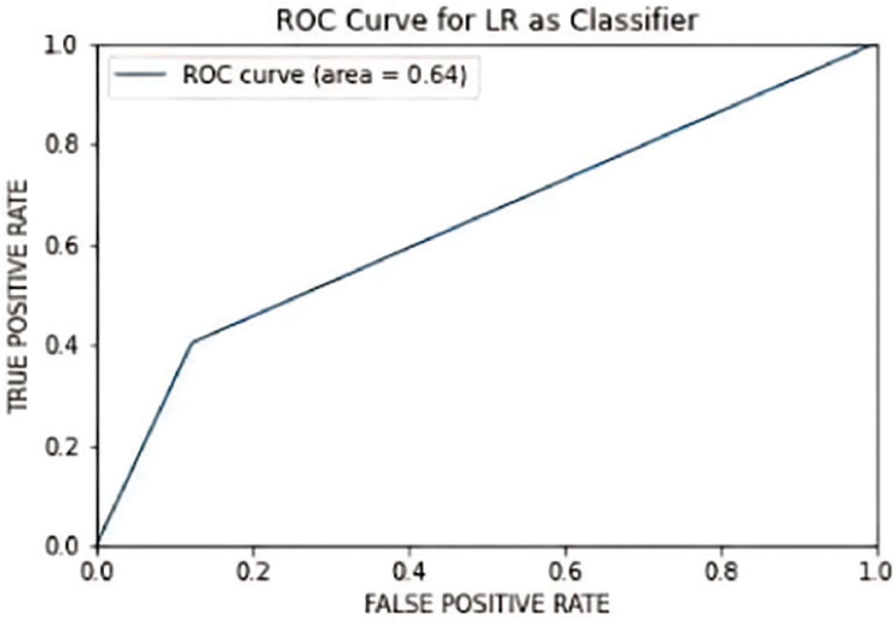
Figure 27:
ROC curve for LR as classifier.
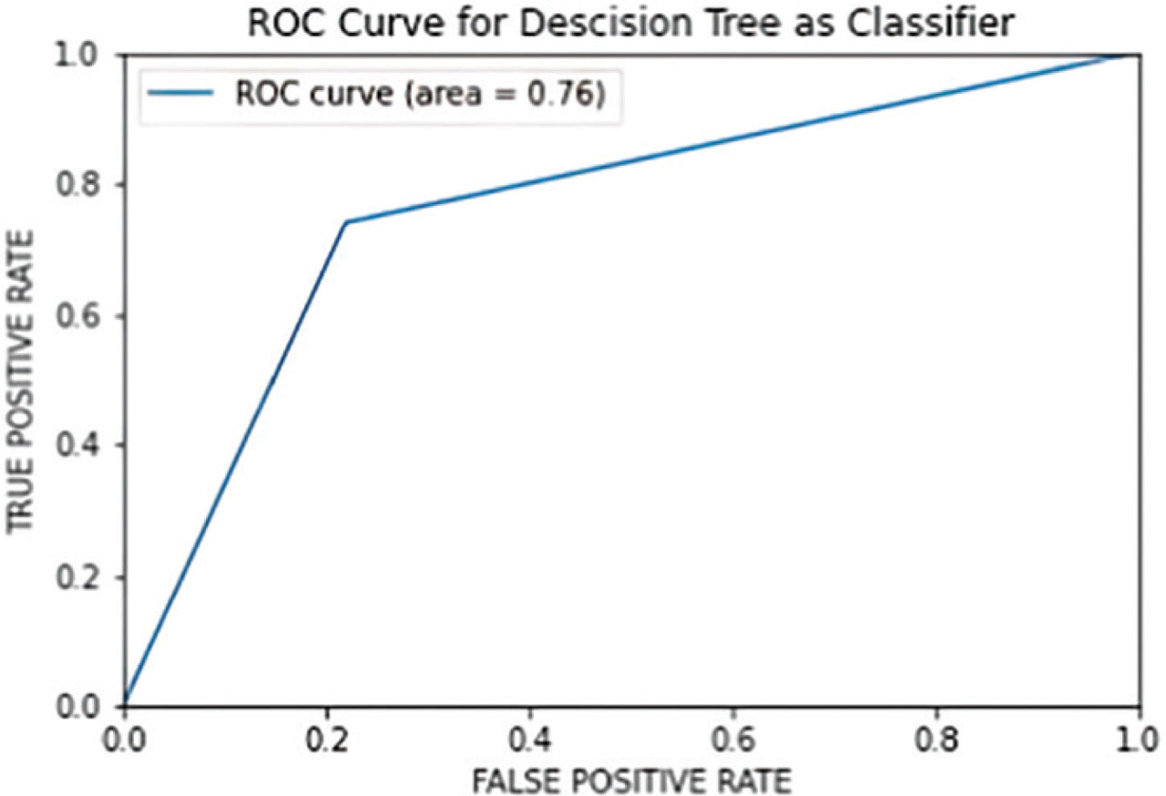
Figure 28:
ROC curve for decision tree as a classifier.
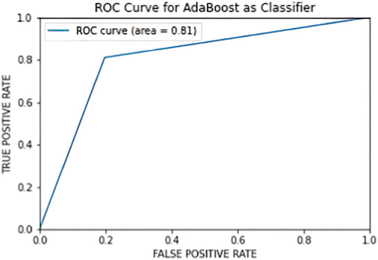
Figure 29:
ROC curve for AdaBoost as classifier.
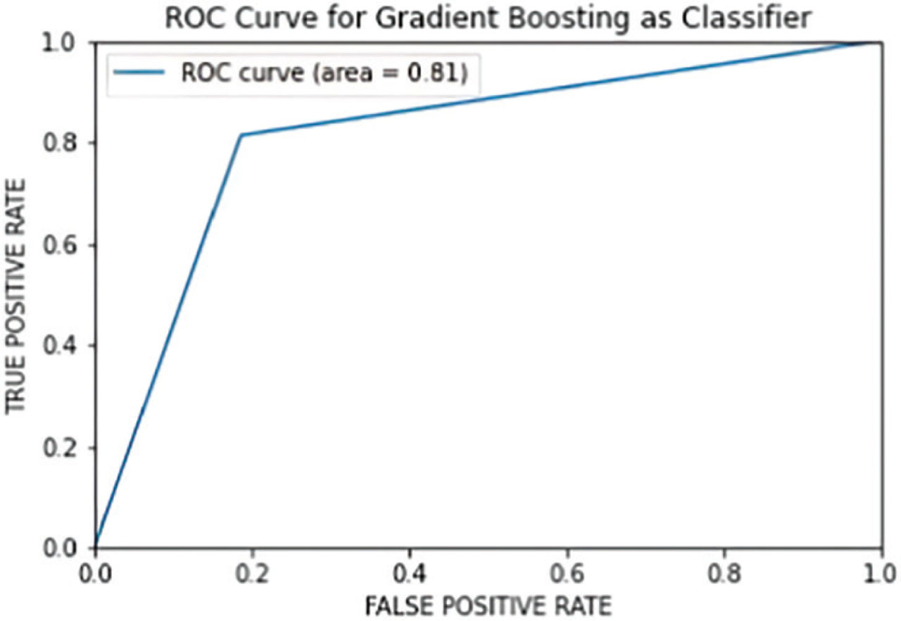
Figure 30:
ROC curve for gradient boosting as classifier.
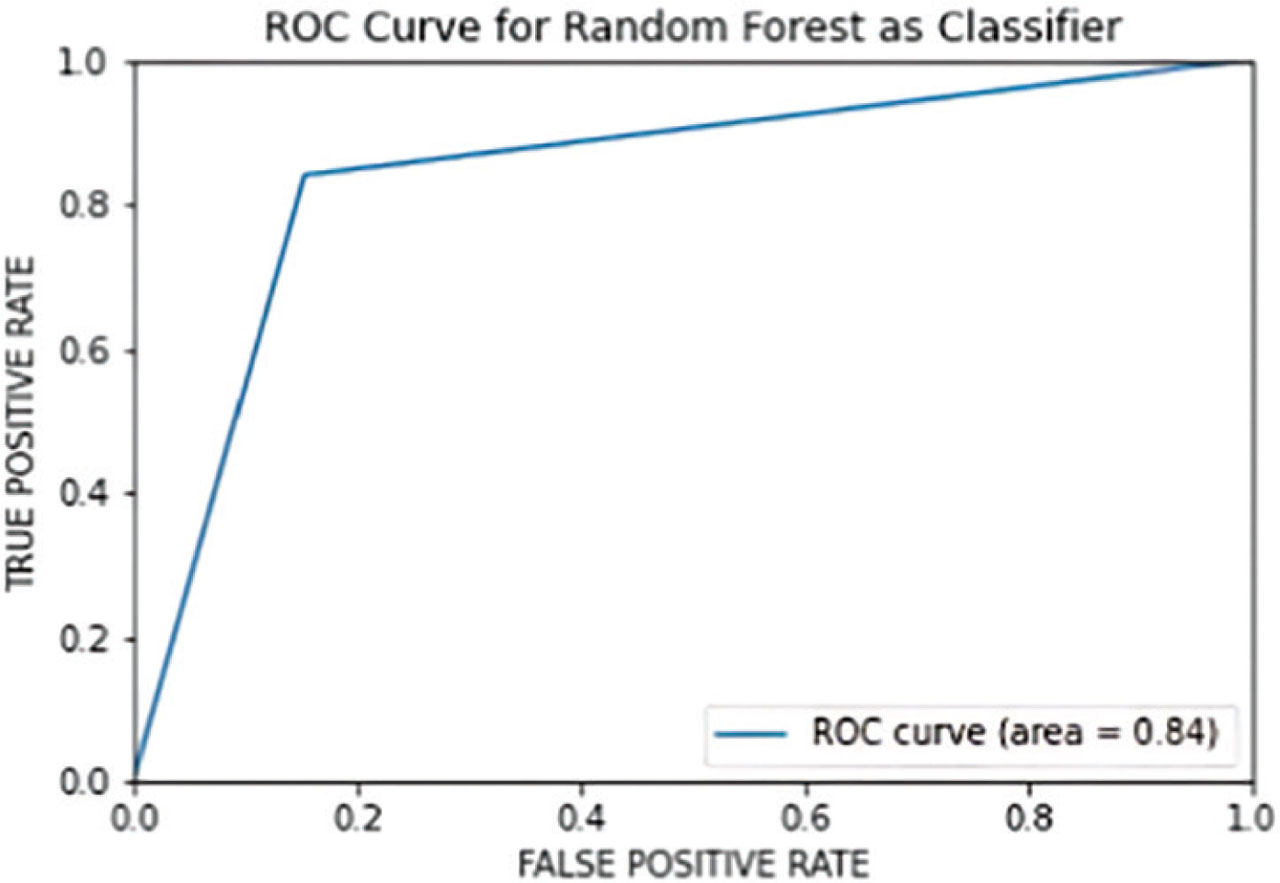
Figure 31:
ROC curve for random forest ensemble classifier.
Table 7:
State-of-the-art methodologies for skin cancer diagnosis
| Study | Dataset | Skin Cancer | Technique | Accuracy (%) |
|---|---|---|---|---|
| I.S. Ali [8] | ISIC 2018 | a, b, c, e, f, h | PGAN | 70.1 |
| R.A. Mehr [10] | ISIC 2019 PAD-UFES-20 | a,b,e | Inception-ResNet-v2 CNN | 94.5±0.9 |
| AQ. Usca [11] | MSCD10000 | a | AlexNet CNN | 91.30 |
| N.M Mahmoud [16] | PH2 | a, b | ANN | 94 |
[i] (a) Melanoma; (b) Melanocytic nevus; (c) Basal cell carcinoma; (d) Benign keratosis; (e) Actinic keratosis; (f) Intraepithelial carcinoma; (g) Dermatofibroma; (h) Vascular lesions; (i) Benign melanocytic lesions; (j) Malignant and pre-malignant keratinocyte carcinoma; (k) Dermatofibroma; (l) Nevus pigmentosus; (m) Squamous cell carcinoma.