
I. Introduction
Melanoma of the skin, a lethal form of skin cancer, originates in melanocytes, the skin cells responsible for producing melanin. This cancer tends to develop in areas of the skin that receive frequent exposure to sunlight. The skin comprises two primary layers: the epidermis and the dermis, with the hypodermis constituting the fatty tissue layer beneath. The epidermis, responsible for continual skin regeneration, is composed of the basal cell layer and the squamous layer. The basal layer contains melanocytes, which produce melanin, a dark pigment that imparts color to the skin. Melanocytes generate melanin as a defense mechanism against skin burns caused by UV radiation. The accumulation of excessive melanin results in the formation of moles, which, in some cases, have a risk of progressing into melanoma. Also referred to as cutaneous melanoma, this type of skin cancer differs from regular moles. Various forms of melanoma exist, including superficial spreading melanoma, nodular melanoma, lentigo malignant melanoma, acral lentiginous melanoma, and desmoplastic melanoma [1]. Typical moles exhibit a uniform color with clear borders, distinguishing them from the surrounding skin. In contrast, melanomas display asymmetry, irregular borders, a larger diameter, uneven color distribution, and may show symptoms such as itchiness or bleeding. They initially appear as small spots that gradually become larger. These spots manifest in various shades and sizes, eventually losing their regular shape and symmetry. Detecting melanoma involves self-examination, particularly monitoring existing moles for any unusual changes in the skin. If suspicion arises, a dermatologist may conduct a dermatoscopy or surface microscopy test for accurate melanoma diagnosis [2]. Skin melanoma is ranked as the 17th most prevalent cancer globally. When considering gender-specific statistics, it is the 13th most common cancer among men and the 15th most common cancer among women. Precise diagnosis of skin melanomas in the early stage is the major challenge faced by doctors. Interpretations of doctors may vary based on experience and knowledge. Dermoscopy has 89% sensitivity in detecting skin cancer and may result in a false diagnosis due to the absence of deterministic dermoscopic features for melanomas [3]. Detecting skin cancer significantly escalates the chances of successful treatment. Artificial intelligence diagnosis tool facilitates the early detection of melanoma cancer, thereby increasing the survival rates of cancer patient. Machine learning (ML) models purposefully built for melanoma detection undergo four key phases, including pre-processing, segmentation, feature selection, and classification. However, the presence of hair and other marks in the images poses a challenge for ML algorithms in the context of skin cancer detection [4]. Recent development of artificial intelligence models such as enhanced super generative adversarial network (ESRGAN) designed for creating a set of authentic enhanced images from the given training image dataset is a new milestone in the domain of medical image processing. This research study aims at developing a novel framework for improving the performance of a simple three-layer CNN model with ESRGAN and enhanced density-based clustering algorithm. The novelty of this research work lies in the framework that includes unique ESRGAN for enhancing the dataset, followed by the density-based clustering algorithm enhanced with swarm salp optimization (DBCESp) for segmentation and custom-built CNN model for melanoma image classification. The unique architecture of ESRGAN included in this framework improves the performance of the model by generating versatile images in the dataset. The dataset is further improved by data augmentation before segmentation and classification. The efficiency of this framework is unlocked when the algorithms of ESRGAN and DBCESp are paired with CNN.
II. Literature Review
Skin cancer is broadly classified as melanoma and non-melanoma skin cancers. Melanoma is a fatal type of cancer with a lower survival rate than non-melanoma cancer. Researchers use the International Skin Imaging Collaboration (ISIC) dataset for skin cancer detection. The examination of pigmented skin lesions adheres to the ABCDE criteria [5] where A stands for Asymmetric shape of lesion, B for Border irregularity, C for Color variability, D for Diameter greater than 6 mm, and E for Evolving characteristic related to the shape and size. Lesions diagnosed can be smaller than 6 mm in certain cases [6]. Multicentric diagnostic study [7] developed a model for special kind of melanoma called melanoma-nevus classification using histopathological whole-slide images from German hospitals, which were analyzed by AI-based classifier. The main challenge of privacy issues in dataset collection is surpassed by federated learning in this study. An accuracy of 70.1% is achieved by progressive generative adversarial networks (PGAN) using a self-attention mechanism for the classification of skin lesion images [8]. A hybrid method of ML and deep learning is adopted for melanoma lesion diagnosis [9]. The Inception ResNet v2 CNN with Adam optimizer and a global learning rate as 0.001 spanned 30 epochs and achieved an accuracy of 94.5% in distinguishing the lesion as between malignant and benign [10]. AlexNet-based CNN is adopted in this study to identify melanoma at an early stage where pre-processing is carried out with morphological algorithm combined with common filtering techniques [11]. CNN-based stacked ensemble framework exhibited an accuracy 95.76% to detect melanoma skin cancer [12]. The effectiveness of the Entropy-aware similarity for balanced clustering method is implemented on actual melanoma medical data to evaluate cluster while preserving balance [13]. The performance of three-dimensional (3D) and two-dimensional (2D) CNN are investigated on a dataset with 1,690 melanocytic lesions, and the diagnostic performance of the CNN was compared with histopathology and dermatologist assessment [14]. The MLP model predicted BRAF mutation alteration status, an important biomarker in predicting melanoma from the patient’s clinical and histological data [15]. A novel framework for skin cancer diagnosis developed with adaptive snake algorithm in duo with region growing algorithm performs ROI segmentation and with ANN as classifier shows an accuracy of 94% [16]. The study shows that for ISIC 2019 and 2020 melanoma dataset, the best reported overall accuracy from the applied CNN experiments is by the MobileNet pre-trained model [17]. The challenges faced by skin melanoma diagnosis are skin lesion segmentation resulting in unclear lesion boundaries, differences in appearance among skin lesions, and color and texture changes according to demography. However, these disadvantages were surpassed with the advent of deep learning models, brightness, shape and artifacts pose serious challenges to accurate diagnosis [18]. According to state-of-the-art studies, deep learning techniques are more efficient in detecting melanoma than traditional ML algorithms. The existing studies deal with all skin cancer types, not just melanoma. The proposed study aims at classifying melanoma images from other normal rashes for medium sized datasets.
III. Deep Learning Algorithm for Medical Image Processing
For decades, medical imaging modalities like computed tomography, X-rays, ultrasounds, and magnetic resonance imaging have played a vital role in extracting accurate information about disease conditions for diagnosing diseases, performing surgery, and treating patients in the healthcare industry. However, challenges in analyzing medical images arise during the image acquisition process. Factors such as the illumination conditions under which images are acquired impact the image contrast and clarity. Additionally, slight movements of patients due to breathing introduce quantum noise in images. There is a need to maintain a trade-off between the radiation dosage given to the patient and the image quality. The quality of the image is affected by noise, blur, and low contrast due to the reduction of the radiation dosage given to patients. To address these challenges, various denoising and contrast enhancement algorithms are applied to clean and enhance medical images [19]. However, these algorithms may sometimes blur vital information, create unrealistic contrast enhancements, and result in noise amplification and excess brightness. Several research studies proclaim that segmenting the region of interest before classification improves the model’s accuracy. The algorithm performance is directly affected by noise, blunt edges, and outliers with intensities like the region of interest. Feature extraction prior to classification is an inevitable task [20]. Study shows that dataset chosen for the study affects the model performance of the ML classifier [21]. The need for labeled datasets and the availability of real-time medical images with skewed labeled distributions are challenging for ML algorithms [22]. Conventional ML algorithms may face overfitting issues, where the model performs well on the training dataset but poorly on the test dataset [23]. Real-time data requires preprocessing and feature reduction before classification or prediction [24]. Therefore, in this research study GAN model is utilized for pre-processing skin images, DBCESp for segmentation, and deep learning for classification. This research study makes an earnest attempt to address the challenges faced in developing an automated diagnosis tool for melanoma diagnosis. This proposed framework leverages the deep-learning techniques for preprocessing as well as classification of the melanoma images. Deep-learning models, such as CNN and ResNet, can discover patterns in medical image data and accurately predict the labeled class for any test sample. Deep learning techniques find wide applications in image processing as they do not require feature engineering, especially with large datasets. Figure 1 shows the block diagram for the proposed deep learning model for melanoma image classification.
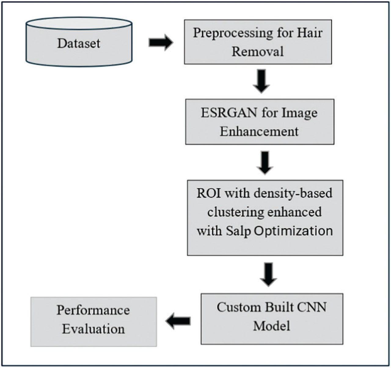
Figure 1:
Block diagram of proposed framework. ESRGAN, Enhanced super generative adversarial network.
IV. Proposed Methodology for Melanoma Cancer Detection with CNN
The proposed framework for melanoma diagnosis includes the preprocessing phase to remove unwanted objects, enhanced super GAN to generate super-resolution images from the low-resolution images, followed by segmentation with a novel algorithm, data augmentation to create a versatile dataset, and finally classification with the CNN.
a. Dataset
The dataset for this study is melanoma skin cancer images from the ISIC. The ISIC 2016 dataset is a standardized public benchmark for high-stakes computer-aided diagnosis in dermatology. The diagnostic labels for the images were rigorously derived from definitive pathology reports for confirmed cases and from the unanimous clinical consensus of multiple experts for the samples. Images are 8-bit JPEGs, but they exhibit extreme variation in spatial resolution. The dataset includes a training dataset of 2,000 images, a testing dataset of 600 images, and a validation dataset of 150 images [25]. The dataset chosen for this study is a publicly available medium-sized dataset. Medium-sized datasets often require less computational power and storage compared to larger datasets. Training deep learning models on smaller datasets takes less time and resources.
b. Pre-processing
Medical images typically require pre-processing before segmentation and classification. The pre-processing phase of the noise removal and image resolution enhancement is the foremost step in any computer-aided diagnosis model. The hair removal is performed with a simple Otsu thresholding method. With the advent of deep learning techniques aiding in improved noise removal and resolution enhancement tasks for images, traditional noise removal methodologies are now obsolete. This study utilizes a super resolution generative adversarial network (SRGAN) to simultaneously remove noise and enhance image resolution, facilitating further processing in the model.
Complex acquisition procedures may introduce slight blurring in images. Therefore, pre-processing in medical diagnostics is crucial for generating high-quality, super-resolution images from lower resolution counterparts. GAN is an artificial intelligence model with a generator and discriminator [26]. The generator generates the samples from the given input, the discriminator validates the truth of the samples, and the model terminates at the point where the generator and discriminator strike a balance.
The following algorithm is for Melanoma image diagnosis with ESRGAN.
Input: Set of low-resolution melanoma images
Step 1: Set the parameters for the Generator and Discriminator models.
Step 2: While <not converged>
Step 2.1: Generate super resolution image.
Step 2.2: Train the discriminator with generated dataset.
Step 2.3: Generate more images with the objective of minimizing loss function.
Step 3: end < while loop >
Step 4: Save the generated images as
Step 5: Calculate the PSNR values for D and D′.
Step 6: Calculate the average of all images in D′. Record the average values as output.
In SRGAN, the generator and the discriminator network work against each other to learn the dataset. The architecture of the generator network includes the initial convolutional layer + PReLU activation layer, a middle layer of residual blocks, and finally the last layer. The main block in GAN is replaced by residual-in-residual dense block (RRDB) [27]. The proposed ESRGAN has three residual blocks in RRDB with five subblocks of plain Conv2D and ReLU stacked together without residual skip connection enables deeper feature extraction compared to the RRDB blocks of SRGAN. The sequential stacks of Conv2D enable non-linear feature composition inside each block and help in learning specific features rather than the conventional GANs. The first convolution layer has number of filters nf and the growth channel gc is 32. The four consecutive layers have number of filters increasing according to the growth channel with the formula nf + i × gc where i is the order of convolution layer within residual block that takes the values i = {1,2,3,4}. The growth channel determines the number of features learnt at each layer. Leaky ReLU is the activation function used that prevents diminishing ReLU problems and preserves the gradient flow. The final fused feature map is scaled by a factor of 0.2 and concatenated to the original input, forming a local residual connection. The forward pass logic creates dense connectivity, stronger gradient flow, stabilizes network learning, and reconstruction of frequency details. In RRDB, the residual learning takes place at multiple levels. Residual scaling scales down the residuals by factor 0 or 1 before entering the main path. Residual blocks retain the information in the previous layers allowing the network to select apt features from the available set of features. The batch normalization (BN) layers are removed as they introduce artifacts and curb the generalization of the model. The BN layer mostly induces artifacts only in deeper networks in GAN model and hence the removal of the BN layer stabilizes the model.
The last layer includes up sampling and Conv2D layer. The output images of RRDB block are upsampled and finally given as input to the convolutional layer. The parameters that control the network complexity include the number of feature maps and growth channel value. The number of feature maps in the Convolution layer is 64 and the growth channel value is 32. Since BN is not used the bias is included. Each Convolution layer has increasing growth channels to employ dense connections. Dense connections improve the gradient flow and help in training deeper networks to learn intricate patterns. The distinctive feature of SRGAN is the perceptual loss function that is developed by constraining the features before activation. The ESRGAN generator creates a novel training dataset for the model from the given training dataset. When features are used after activation there is inconsistent brightness due to reconstruction and leads to poor performance. The discriminator in this model is defined as realistic average discriminator. Introducing network interpolation avoids introducing artifacts and balances perceptual quality without retraining the model. Figure 2 shows the architecture of ESRGAN.
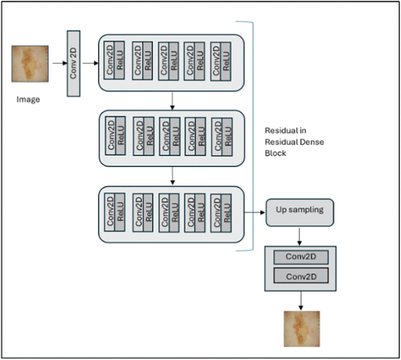
Figure 2:
Architecture of ESRGAN. ESRGAN, enhanced super generative adversarial network.
Data augmentation is a highly effective pre-processing technique for improving model performance in ML. Data augmentation is employed to enhance the generalization and robustness of a ML model, especially in scenarios where the training data lacks diversity. This process involves generating augmented input samples by applying transformations to the original data, thereby improving the model’s adaptability to generalize unseen data. Various augmentation techniques contribute to this process, including flipping, color augmentation, cropping, rotating, shifting, translation, brightness and contrast enhancement, color jittering, noise injection, and shear transformation. Flipping images occurs along either the vertical or horizontal axis, creating variations in the dataset. Color augmentation involves separating a channel of a particular color from the RGB channel, with the matrix of the required channel isolated and the other two channel matrix values filled with zeros. Cropping focuses on extracting the dominant patch of an image along its height and width. Rotating images in a range of 0–360 degrees introduce diversity in the image features. Shifting images upwards and downwards further diversifies the dataset. These techniques collectively enhance the richness and diversity of the training data, fostering improved model performance and adaptability [28]. Figure 3 shows the ESRGAN output of the sample images.
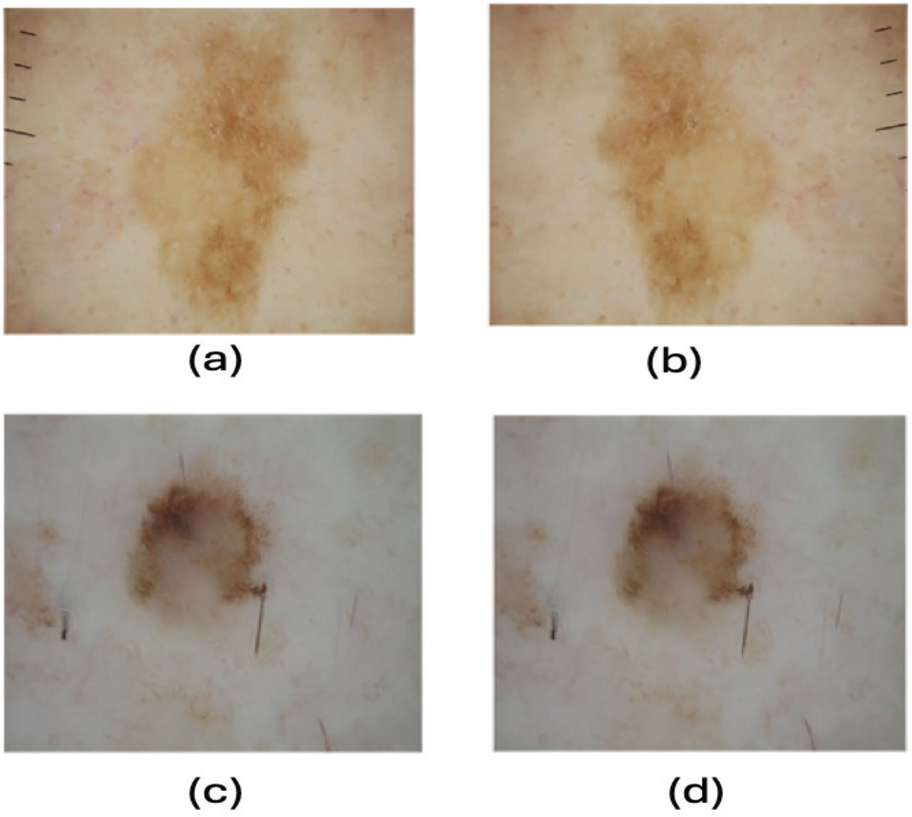
Figure 3:
(A) and (C) Original melanoma images and (B) and (D) the ESRGAN output images. ESRGAN, enhanced super generative adversarial network.
c. ROI segmentation
ROI segmentation is demarcating the regions having distinguished and distinctive features of the image. Primitive ROI segmentation methods like thresholding, edge detection, and region growing are methods based on the pixel intensity of the image. A more sophisticated segmentation method based on unsupervised ML is the clustering method. Soft clustering algorithms cluster the data points in space according to their degree of similarity [29]. Density-based clustering, a popular clustering technique in data science, is adopted in this research study to cluster pixels of similar intensity. This algorithm is based on the ɛ-neighborhood concept in Topology. The ɛ-neighborhood of p is the set of data points {p1, p2, p3,… pn } within a circle of radius ɛ centered at p. For a 2D space, the ɛ-neighborhood is a circle, and in a 3D space, the ɛ-neighborhood is a sphere. Reducing the radius of the neighborhood generates smaller cluster groups of data points. The algorithm computes dense clusters of similar datapoints with smaller radii. The density-based clustering non-parametric algorithm (DBSCAN) algorithm focuses on two parameters: the radius of the neighborhood and the minimum threshold of data points present in the cluster. Every point in the data-space is categorized as a core point, border point, or outliers. A data point is a core point if the neighborhood is a potential cluster member point. If two points p1 and p2 are said to be connected if there is a point p12 which is reachable from point p1 and p2. The border point is any point directly reachable from the core point or by transitive closure property. An outlier is a datapoint that cannot be part of the cluster, as well as cannot change its status as a border point. Core points are selected based on the minimum threshold of points in the neighborhood, hence by altering this parameter, the clusters can be fine-tuned. The DBSCAN algorithm starts with any arbitrary point p and identifies the set of density-reachable points from p by examining the p’s direct and indirect neighbors. If the new point is a core point, then it is directly assigned as part of the cluster. If the point is the border point, then it may be added to the cluster by indirect reachability property. If the point is an outlier, then it is labeled as noise [30]. The clustering solutions of density-based clustering converge toward the local optima. The extended search strategy by the Salp Optimization algorithm overcomes this setback. The algorithm discovers the set of potential core points using its unique search strategy and fitness criteria. Salp is a semi-transparent barrel-shaped marine species from the family of sea squirts. They move as a group like a linear curve in the ocean. In heavy oceans, they form a chain following the leader. All the Salps except the leaders are followers. Like any swarm optimization technique, the position of Salp is defined in the n-dimensional space. Salp aims to find the food source {Fi } in the search space. Mathematically, the leader position in the matrix is updated using Eq. (1):
where {Fi } is food source in the search space. {ubi, lbi } upper and lower boundaries set limits. {cf1,cf2,cf3}are constant values that maintain balance between exploitation and exploration and are calculated by the formula Eq. (2). where t is the current iteration and max_iter is the maximum number of iterations.Salp follower positions are updated by the initial position, swarm movement speed, and acceleration given in the Eq. (3).
where is the position of kth follower Salp in the ith position in the matrix.a = v0 / vf is the acceleration where v0 and vf are initial and final speed, respectively [31]. Density-based clustering algorithm enhanced with Swarm Salp optimization technique (DBCESp) segments the region of interest in the melanoma skin images. After each iteration, the optimum solution is saved as the food source, and the leader position is updated as a function of the food source to converge to the best solution at the end of all iterations. The algorithm always works in and around the best solution. Setting the initial leader position as the core point of the cluster space and finding the ɛ-neighborhood eliminates the risk of Salp optimization converging quickly to the local optimum solution. The search space is extended with the update function having the lower and upper bound parameters restricted by the Euclidean distance as the fitness function between the cluster center and the newly generated Salp population. The proposed DBCESp algorithm for region of interest segmentation in the melanoma skin images is listed below.
Step 1: Read the skin image as Img.
Step 2: Perform hair removal for the image Img. Set parameters radius ρ = size/4 and max_iter = 50.
Step 3: Create a pixel intensity array I of Img.
Step 4: Sort {I0, I1, I2,…Isz } ∀ {I0, < I2 < I3…. < Isz} are unique non-zero values. Find the midpoint m of the array Iarr.
Step 5: Find mean intensity .
Step 6: Create If = {I0, I1, I2,…Im }. Calculate the mean value μf with (4).
Create Is = {Im+1, Im+2,…Isz}. Calculate the mean value μs with (5).
Step 7: Find pixel position {Pf } with intensity rounded off to μf. Mark as core point of the cluster C1. Find pixel position {Ps } with intensity rounded off to μs. Mark as core point of the cluster C1.
Step 8: For each Cluster Ci call the method SalpOptAlgo (Ci,max_iter).
Step 9: SalpOptAlgo (Ci,max_iter)
Step 9.1: while (k < max_iter) for each population
Find all n directly reachable set of points {p1, p2, p3….pn } for Ci from .
Set leadership position with (6).
where lij : set of reachable points from core point .The leader positions are updated with (7).
The position of follower Salp Si are updated with (8).
Calculate the fitness value Fs of each Salp population with (9).
where (xi, yi) is the position of the Salp Si and (xc, yc) is the cluster center.
Step 10: Segment the region of interest with computed final cluster centers.
The DBCESp algorithm is an enhanced version of basic density-based clustering algorithm that needs manual setting of the parameters, such as the cluster center, radius of the cluster, and number of points included in the cluster. The ability to select the optimal values can lead to poor clustering. Salp Optimization is used to optimize these parameters. The fitness function given in the Salp optimization algorithm optimizes the cluster center for segmentation of the region of interest. The algorithm reads the images in the dataset. The intensity of all the pixels in the image is sorted, and the mean intensity is calculated. The image is broadly clustered into clusters based on the intensity.
Each cluster region is now considered for further image processing. The core point Ci of clusters is computed by the Salp Optimization algorithm. The initial search space for the Salp optimization algorithm is the ɛ-neighborhood of cluster centers, the set of data points {p1, p2, p3,….pn } within a circle of radius ɛ centered at C1. The leadership position is updated with the Eq. (7). The position of follower Salp S is updated with the Eq. (8). The fitness value of the Salp population is computed with the Euclidean distance between the Salp population and the cluster center. After the optimal cluster center is identified, the region of interest is clustered from the image.
d. Classification
The structure of CNN includes the input layer, convolutional layer, pooling layer, non-linear activation layer, and fully connected layer. The input layer resizes the images for further processing by the convolutional layer. The images are converted to a standard size in the input layer. The first layer of the CNN model is the convolutional layer with several convolution filters. The input images are convolved with filters to generate feature maps. The multiple convolutional layers in the CNN uncover the unique features such as textures, lines, and curves, and the deeper layers unearth the fine features in the images. Convolution is a mathematical operation that performs an intersection or overlap operation between the two regions f and g given as Eq. (10).
Images are represented as discrete functions f (x, y) and g(x, y). The convolution of two functions representing 2D space is given as Eq. (11).
In any color image, each pixel has intensity values in RGB channel therefore, the input is a multi-dimensional array with 3 × size of the image. For the 2D array, the convolution function is Eq. (12).
Integral form of Z (x, y) is given as
If the convolution kernel size is m × n then Eq. (13) is written as Eq. (14).
The convolution kernel is a square matrix of odd size with discrete values representing weights. The color input image is of size m × m × r where m is the width and height whereas r is the depth. In color images, the depth value r represents the three channels. The kernel slides over the entire image both in the horizontal and vertical direction. The sum of the dot product of the input image and kernel is computed, and then the values are summed up to create a single scalar value and fill the corresponding value in the output feature map. The kernel size in the Convolutional layer is defined as n × n × p, where n < m and p < = r. The convolution layer computes the dot product of the input image and the kernel weights. The output feature map is hk = (Wk × x + bk) [32] where bk is the bias and Wk is the weight. Figure 4 exhibits the architecture of the CNN deep learning neural network for melanoma image classification and diagnosis. The proposed CNN is three layers of Conv 2D blocks followed by flattened layer and fully connected layer. Feature maps are representations of precise input features, and minor changes in the images can alter the feature maps. Image downsampling addresses this issue of minor changes in the images. The pooling layer plays a crucial role in downsampling and feature reduction, effectively reducing network complexity by minimizing the number of convolutional layers. Max pooling highlights the discriminating features and eliminates the background effects. Max pooling, being a non-linear operator, enhances the overall non-linearity of the network. Max pooling prioritizes the neurons with strong activation output, contributing to improved feature extraction [33]. In the CNN model, the flattening layer converts the multi-dimensional output of the preceding convolutional and pooling layers into a one-dimensional array. The unsaturated non-linear activation function ReLU is recommended over functions that cause low convergence speed and gradient dispersion problems. The ReLU activation function is commonly used in deep learning models due to its high convergence speed and simplicity [34]. The main advantage of ReLU activation functions is to learn abstract features through non-linear transformations. The features extracted from images by the convolutional and pooling layers serve as the input to the fully connected layer, which is dedicated to prediction or classification [35]. The selection of the activation function depends on the classification task, whether binary or multiclass. The SoftMax function is the preferred activation function for the prediction that normalizes the output real values to labeled classes in multiclass single-class classifications. Sigmoid function is preferred for binary classification problems such as benign and malignant medical image classifications [36].
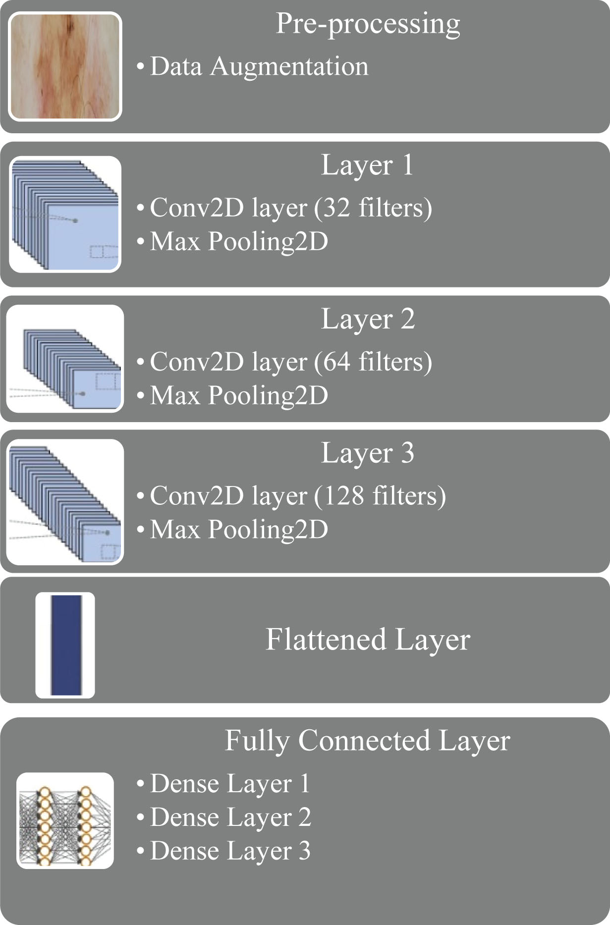
Figure 4:
Architecture of 3-layer CNN model.
V. Results and Discussions
The proposed framework is evaluated experimentally, and the results are tabulated. The high-resolution images are generated by ESRGAN. The resolution change in images by the ESRGAN is experimentally studied with a set of sample images randomly selected from the dataset. Peak signal noise ratio (PSNR) measures the image quality of the generated images to input images fed to ESRGAN model. Another metric for evaluation of the ESRGAN performance is structural similarity index measurement (SSIM). SSIM is a measure of luminance, contrast, and structural information. A higher value of the SSIM metric indicates that the image quality is enhanced compared to the original input image. The PSNR and SSIM values of around one hundred randomly selected images are experimentally evaluated and studied. The experimental results exhibit an average of 38.5 PSNR values. The experimental results show that the SSIM value is on average 0.71 for the generated images with the original images given as reference. The PSNR value recorded for sample images shows that ESRGAN improves the image resolution to an acceptable level [37]. In the proposed segmentation method with DBCESp, the parameters are set to accurately segment the ROI area in the image. The Salp population depends on the search space dimension. Hence, the number of search agents in this Salp swarm algorithm is set to the number of reachable neighbor points within the ε neighborhood of radius ρ. The number of maximum iterations is set as 50, which is a typical value selected for optimization problems. An iteration value higher than 50 will lead to higher computation cost and a lower value will result in quick convergence. The upper and lower bounds are problem-specific and are set to the maximum and minimum pixel intensity in the image. The two clusters segment the image as the ROI and surrounding skin area. The CNN model is built with customized architecture with three Conv2D layers followed by flattened layer and a dense layer. The model has three convolution blocks followed by a fully connected module for classification. Each convolution block has a convolution layer, ReLU activation function, and a 2 × 2 max pooling layers. The convolution block is responsible for extracting hierarchical features, starting from low-level textures to high-level melanoma-specific patterns such as asymmetry, pigment networks, and border irregularities. The first convolution block has 16 convolution filters with ReLU as an activation function and extracts low-level features such as edges, color gradients, and simple textures. The input shape is 224 × 224 × 3. The second Conv2D block has 32 convolution filters with ReLU as activation function. This block extracts lesion attributes, including irregular patterns and multi-tone pigmentations. The third Conv2D block has 64 convolution filters with ReLU as an activation function to learn high-level discriminative features such as asymmetry and border irregularity. The model has a flattened layer of size 1 × 50176 followed by dense layers. Following the convolutional layers, the output feature maps are flattened and then given as input to the fully connected layers. The dense layer has 128 units with ReLU as an activation function, and the last output dense layer has one output unit with sigmoid as activation function. The optimizer for the model is Adam, and the optimizer learning rate is 0.002. Adam is chosen as optimizer as it integrates SGD and RmsProp providing a trade-off between convergence speed and adaptability. Adam is selected as optimizer due to robust hyperparameter tuning, adaptive learning rates, fast convergence, and wide use in deep learning neural networks. In this deep neural network model, Adam converges faster than SGD and is thus computationally more efficient. All experiments were performed on the Windows 10 operating system with 500 GB SSD, 64-bit 8 GB RAM, and Intel i7 10th Gen chip. The CNN model was implemented using Google Collab GPU resources. The programming language used is Python3 and the deep learning libraries of TensorFlow. Figure 5 shows the model summary of the proposed tool for melanoma diagnosis.
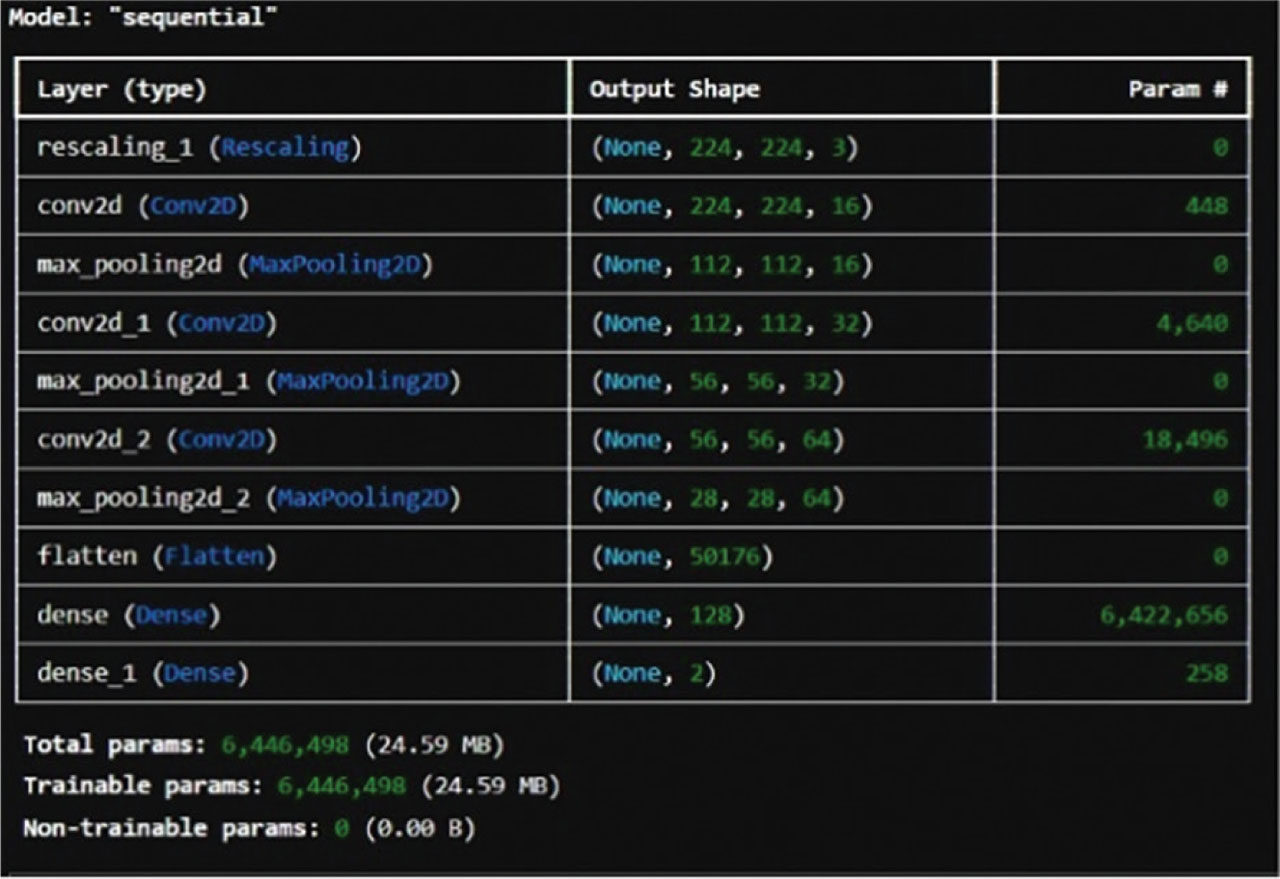
Figure 5:
Model summary for melanoma diagnosis.
The precision value, recall rate, and accuracy value are recorded in this table. The formula for precision, recall rate, and accuracy is given in Eqs. (15)–(17) where TP is true positive, FP is false positive, TN is true negative, and FN is false negative.
Table 1 is the experimental results of five various models for melanoma diagnosis. The 1stCNN model is a simple three-layer model built as per Figure 5. The model has no BN or dropout layers and exhibits an accuracy of 75.5%.
Table 1:
Experimental results of the model proposed for melanoma image diagnosis
| Classifiers | Precision (%) | Recall (%) | F1-score (%) | Accuracy (%) |
|---|---|---|---|---|
| CNN model | 74.3 | 78.5 | 75.7 | 76.4 |
| CNN model with augmentation | 87 | 91.2 | 89.5 | 89 |
| ESRGAN + CNN | 92.9 | 91.6 | 92.3 | 92.2 |
| DBCESp + CNN | 90.4 | 91.2 | 91.0 | 91.0 |
| ESRGAN + DBCESp + CNN | 94.6 | 94.3 | 94.5 | 94.5 |
The 2nd model is a three-layer CNN model with augmentation phase added. The model shows improved performance compared to the CNN model with the accuracy score increased to 89.5%. The 3rd model is ESRGAN, followed by three-layer CNN. The model shows improved accuracy than the other previous models. The fourth model is a three-layer CNN with input images segmented by the DBCESp algorithm without ESRGAN. The performance is at par with the ESRGAN and CNN models. The last model is the proposed ESRGAN-DBCESp-CNN model, which shows improved performance compared to all the previous models. In the performance evaluation, the recall rate, also known as sensitivity, is a metric that measures the model’s ability to classify the samples in the dataset accurately with no misclassifications. High recall indicates that the model detects most of the true positives in the dataset. In medical diagnosis, missing even a negligible number of positive cases proves to be a fatal error; hence, identifying the positive instances accurately is crucial in disease diagnosis. The recall rate is highest for the proposed model, indicating that all the previous models have a considerable number of false negatives in the diagnosis. Figure 6 showcases the confusion matrix of the simple three-layer CNN model without augmentation, or SRGAN-DBCESp-CNN. The accuracy of the basic three-layer CNN model is 75.7%. Figure 7 shows the confusion matrix of the CNN with augmentation phase. Augmentation plays an important role in any deep learning network. The number of false positives is reduced from 81 to 39, and false negatives are reduced from 64 to 24 in the diagnostic results with the augmentation phase. The marked increase in the recall rate and precision indicates the significance of including augmentation as a pre-processing phase. Data augmentation has improved the model by increasing the diversity of the training dataset. Figure 8 shows the confusion matrix with ESRGAN and CNN. The CNN model enhanced by ESRGAN and augmentation has reduced the false positive count from 39 to 21, whereas the false negative count is the almost same. With the decrease in false positives, the model has shown an increase in the F1-score and precision rate. ESRGAN generates high-resolution images that aid the model make precise diagnosis of the melanoma images. The accuracy and recall rate of the CNN model with ESRGAN is 92.3.5% and 91.6% for diagnosing melanoma images. Figure 9 exhibits the confusion matrix for models with CNN and DBCESp Algorithm. In this model the images are segmented by the DBCESp algorithm and given as input to the three-layer CNN model with augmentation phase has shown increase in the false positive count and thereby reducing the F1-score. This clearly indicates the role of ESRGAN in the proposed framework in increasing the model performance. Figure 10 exhibits the confusion matrix of proposed framework. The experimental results indicate a decrease in the false positive count and false negative count, improving the model performance significantly. The proposed framework with ESRGAN, DBCESp, and the custom-built CNN model, including augmentation phase, shows the best classification performance compared to all the CNN models. The marked improvement in the precision shows that the false positives have dropped compared to the basic CNN models. False negative rate is also reduced, and hence the recall rates have increased. The ESRGAN-DBCESp-CNN model has 94.5% accuracy, 94.3% recall rate and 94.5% F1 score. Experimental results strongly imply that most of the images in the test data are accurately classified without many misclassifications.
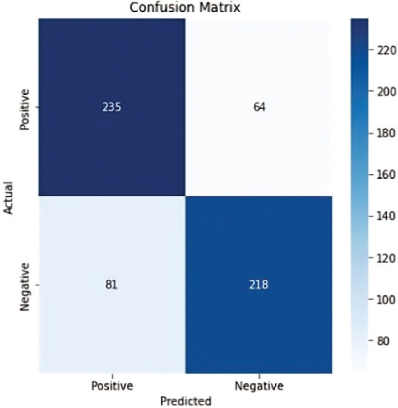
Figure 6:
Confusion matrix for simple three-layer CNN model without augmentation.
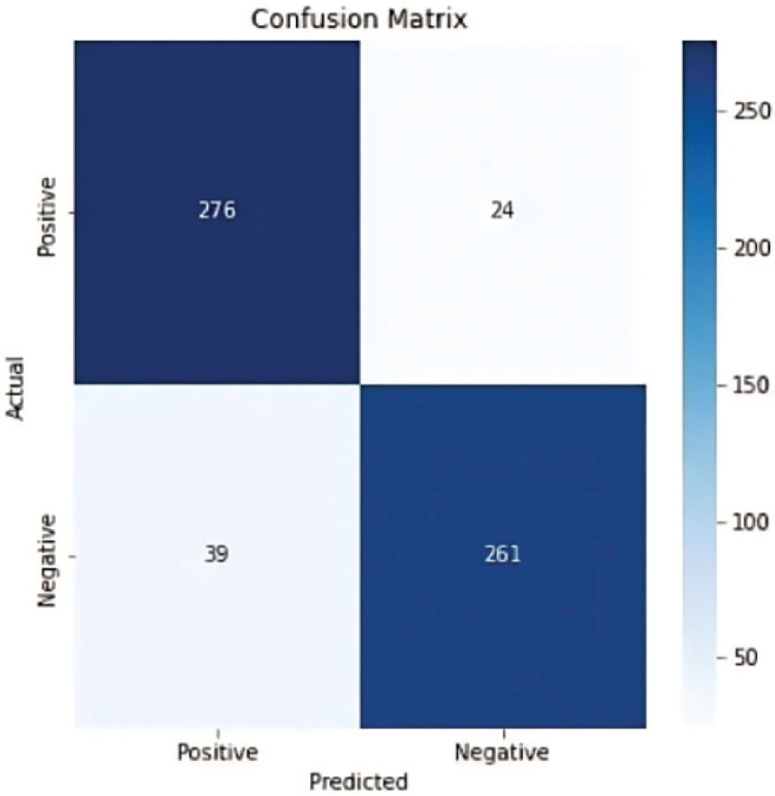
Figure 7:
Confusion matrix for CNN model with augmentation.
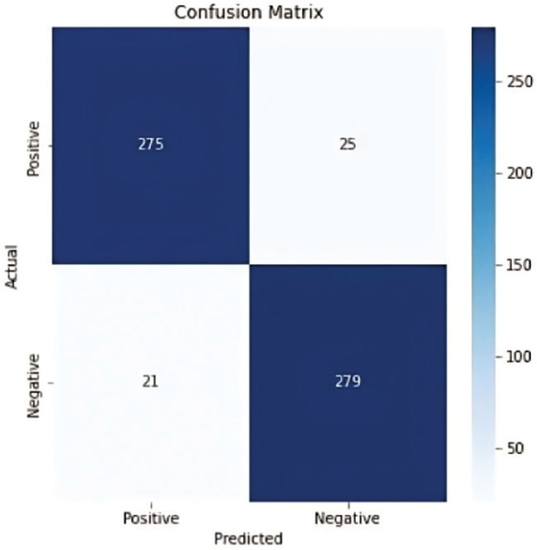
Figure 8:
Confusion matrix for model with CNN and ESRGAN. ESRGAN, enhanced super generative adversarial network.
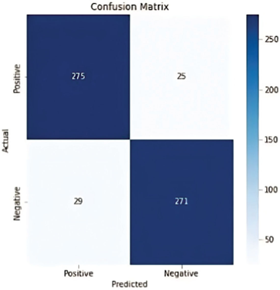
Figure 9:
Confusion matrix for model with CNN and DBCESp algorithm.
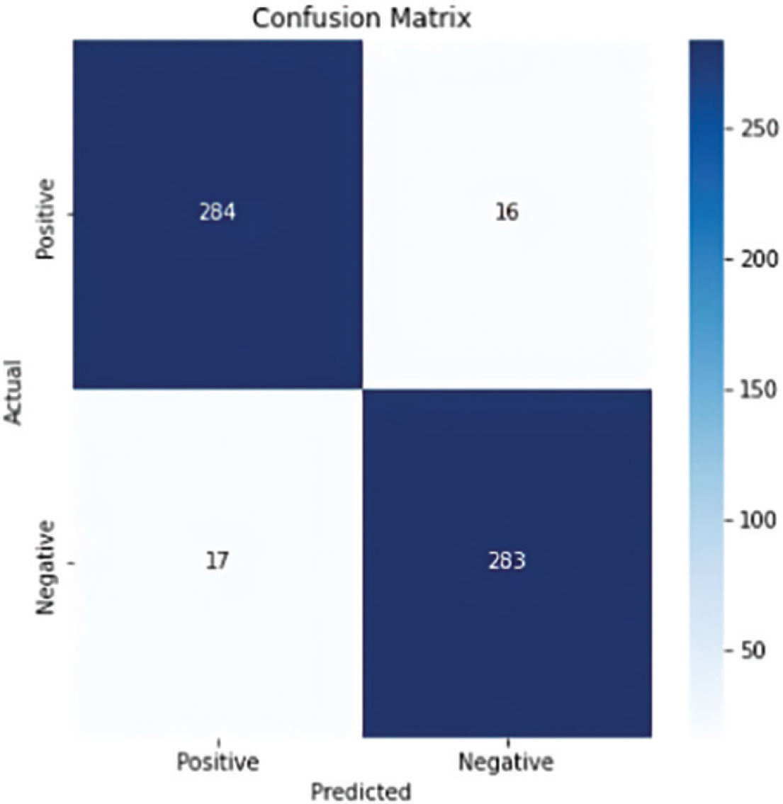
Figure 10:
Confusion matrix for melanoma diagnosis with proposed ESRGAN-DBCESp-CNN model. ESRGAN, enhanced super generative adversarial network.
The experimental results show high accuracy due to ESRGAN. ESRGAN can reduce overfitting indirect ways. Under normal circumstances, CNN tries to learn spurious patterns and learn from irrelevant pixels found in noisy data with artifacts. Overfitting issues are less in a model when the data is less noisy. ESRGAN produces image sets that have high resolution, clearer boundaries, and consistent textures. A CNN trained on pre-processed enhanced images learn the lesion features better compared to raw images. CNN demands deeper layers when the input images are of low quality. ESRGAN, as a pre-processing module with a shallow CNN, performs at par with CNN with deep layers. Moreover, data that has clear class separation can lead to better generalization. ESRGAN produces clear images that lead to reduced gradient noise and, in turn, improve stability. The feature enhancement by ESRGAN improves the regularization of CNN model.
The training and validation accuracy curve shows the number of epochs on the x-axis and accuracy rate along the y-axis. The accuracy curve shows the ratio of correctly classified samples to the total number of samples. The accuracy curve that begins at zero and steadily increases indicates that the model learns the data patterns well. A smooth learning curve implies that there is a gradual change in the model performance while training. Figure 11 shows the training and validation accuracy curve for the CNN model. The validation curve is found to be zig-zag with sharp changes. These sharp zig-zag curves are called unstable learning curves. Validation accuracy fluctuations indicate that the model corrects itself repeatedly and has overfitting issues. The three-layer CNN model is a simple architecture without augmentation or preprocessing phase. Figure 12 exhibits the training and validation graphs per epoch for the ESRGAN and CNN model. The reason for the validation curve to fluctuate validation data being noisy and small. The sharp zig-zag pattern of the validation curve has improved in Figure 12. Though the dataset was medium-sized, the images generated by data augmentation and ESRGAN have played a vital role in improving the classification model.
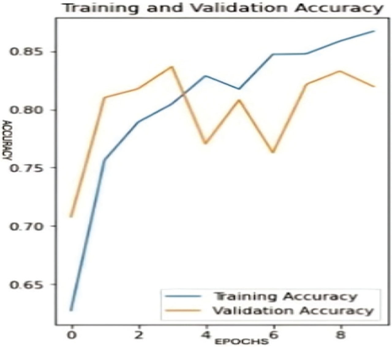
Figure 11:
Training and validation accuracy graph per Epochs for the simple CNN model.
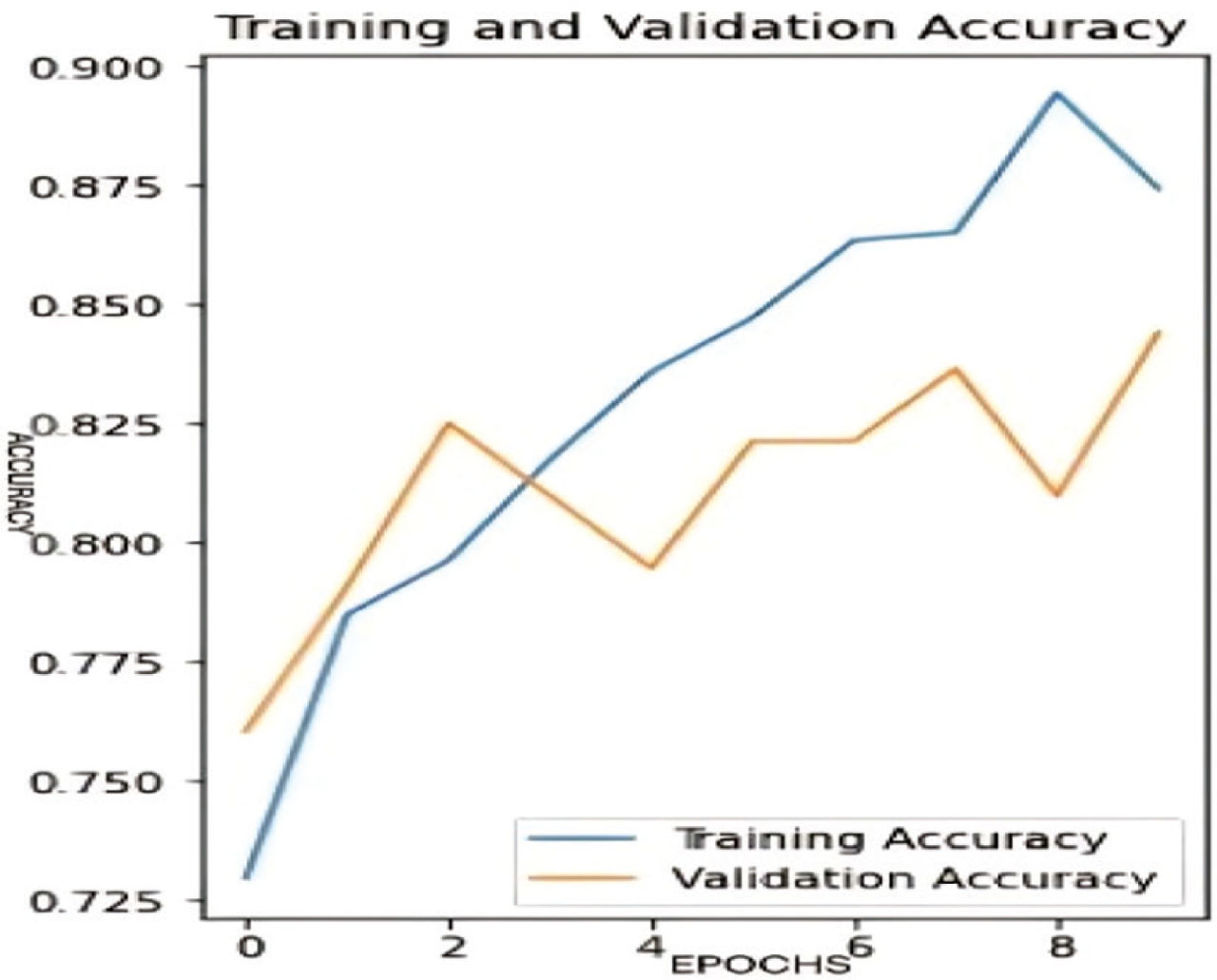
Figure 12:
Training and validation accuracy graph per epochs for the CNN model with ESRGAN. ESRGAN, enhanced super generative adversarial network.
Figure 13 shows the training and validation accuracy graph for ESRGAN-DBCESp-CNN model. The smooth increase in the learning curve and absence of zig-zag pattern in the initial part of the validation curve indicate that the model learns meaningful patterns from the training data. Validation performance shows improvement as the model generalizes to new data. The pre-processing phase of the framework has improved the model performance, and this is evident from the accuracy and validation graph presented. Based on the experimental results, we can summarize that in any classification model, preprocessing is a significant phase that directly impacts the classifier performance. This research paper enhances the simple customized CNN model with pre-processed melanoma images. Any sophisticated deep learning model demands a high-volume dataset, which incurs high computation cost and resource requirements. This research study emphasizes the importance of preprocessing before classification to improve the performance of a simple three-layer CNN model. Table 2 exhibits the time complexity of DBCESp algorithm. This section analyses the time complexity of DBCESp algorithm. It is then compared to the Fuzzy c-means clustering algorithm to show that DBCESP algorithm complexity is better compared to FCM. The neighborhood search with spatial indexing method results in O(nlog n). The time complexity for visiting each data point and assigning it to clusters is O(n). In the Salp optimization algorithm for generation of the Salps and evaluating their fitness gives a complexity of O(p.n), where p is the number of Salps and n is the number of data points. The complexity for updating the Salp positions and evaluation of the fitness function for each new solution is O(I.p.n), where I specify the number of iterations. The total time complexity of the DBCESp algorithm is O(nlog n) + O(I.p.n). Table 3 and Table 4 show the time complexity of DBCESp algorithm and Fuzzy C-means clustering algorithm.
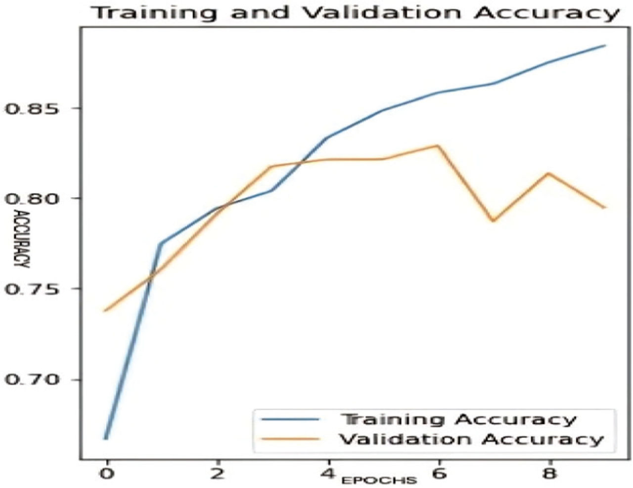
Figure 13:
Training and validation accuracy graph for ESRGAN-DBCESp-CNN framework. ESRGAN, enhanced super generative adversarial network.
Table 2:
Time complexity of DBCESp algorithm
| Steps | Complexity |
|---|---|
| Neighborhood search | O(nlog n) |
| Cluster formation | O(n) |
| Salp optimization - evaluating fitness | O(p.n) |
| Update Salp position and evaluate fitness of new solution with I iterations | O(I. p.n) |
| Total complexity | O(nlog n) + O(I. p.n) |
Table 3:
Time complexity of fuzzy C-means clustering algorithm
| Steps | Complexity |
|---|---|
| Initialization of membership matrix (m, n) | O(mn) |
| Compute cluster membership for each data point | O(m.n.d) |
| Cluster center updations | O(m.n.d) |
| Stop criteria | O(m.n) |
| Salp optimization algorithm | O(I. p.c) |
| Total complexity | O(m.n.d) + O(I. p.c) |
Table 4:
Performance evaluation of the four-layer CNN models
| Classifiers | Precision | Recall | F1-score | Accuracy |
|---|---|---|---|---|
| Four-layer CNN | 80.9% | 79.5% | 80.2% | 80.43% |
| Four-layer CNN model with BN and dropouts | 88.1% | 68.8% | 74.7% | 78.0% |
Melanoma diagnosis with proposed framework of ESRGAN-DBCESp-CNN model shows improved performance compared to the other models listed in Table 1. The dataset includes low-resolution images at different lighting variations with artifacts. ESRGAN included in the proposed model, plays a crucial role in reducing artifacts and improving the resolution of the images. The melanoma diagnosis relies on the fine details in the images, such as the irregular borders, color variations, and small pigment changes. Diagnostic features are highlighted with the ESRGAN, increasing the image resolution preserving the high-frequency details. Considering the proven fact that better inputs give better outputs, high-resolution images provide higher diagnostic performance for simple CNN networks. CNN extracts the low-level features such as edges and textures, mid-level features such as patterns and shapes, as well as high-level features such as lesion characteristics, which are significant for improving diagnostic performance. ESRGAN improves the edges and textures of the images as well as the local contrast, thereby improving feature maps and the overall classification accuracy.
VI. Comparative Study with other CNN Models
The model is compared to the four-layer CNN model with and without BN and dropout layers. The four-layer model includes four Conv2D layers with max pooling layers in between. The convolution layer is followed by a flattened layer. There are three dense layers in the model with unit parameters 62, 128, and 256 with ReLU as activation function. The last layer has the activation function as sigmoid that predicts the output. The optimizer used in this model is Adam. The four-layer model is altered by introducing BN and dropouts. Figure 14 is the summary of a four-layer CNN model without BN and dropouts. Figure 15 shows the summary of the altered CNN model with BN. The BN layer is included in every Conv2D block along with a dropout layer. The weights of the dropout layers are 0.2, 0.3, 0.4, and 0.5 for each Conv2D block, increasing with the number of units in Conv2D block. The experimental results of four-layer CNN architecture without BN and dropouts and with BN and CNN are recorded in Table 4.
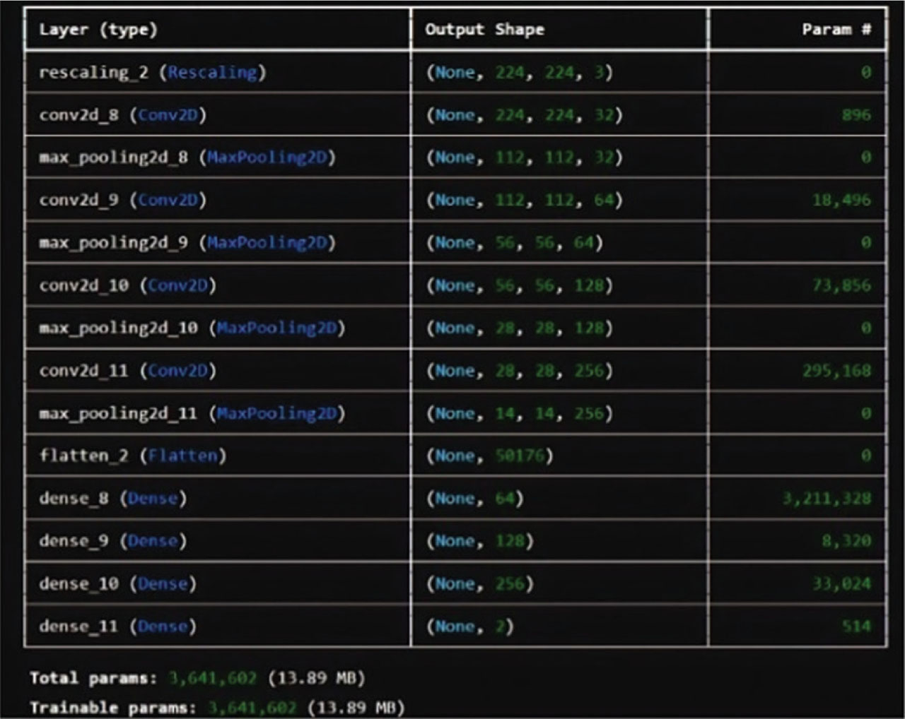
Figure 14:
Summary of four-layer CNN model without BN and dropouts. BN, batch normalization.
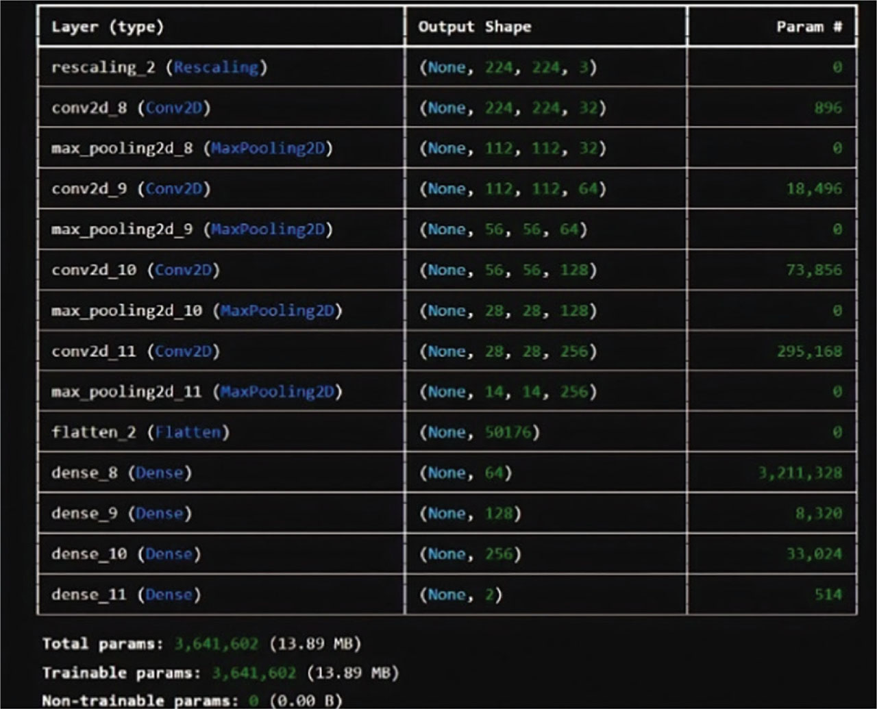
Figure 15:
Summary of four-layer CNN model with BN and dropouts. BN, batch normalization.
Figure 16 shows the training and validation accuracy graph for four-layer CNN model without BN and dropout layers. The learning curve in Figure 16 shows smooth increase in the accuracy, whereas the learning curve in Figure 17 shows that curve starts learning at a high accuracy due to BN and dropout layer. This is a clear indication of overfitting risks involved. In Figure 17, the validation curve shows an inverse hyperbolic curve with three stages. Initially, the model exhibits high validation performance but gradually decreases and at a particular point starts to increase. This condition occurs when the model is too sophisticated for the dataset. The model learns the dataset well in the training phase but is unable to perform well for validation dataset. Accidentally the model hits high accuracy at initial stage but degrades as the number epochs increases. These experimental results indicate that for a medium sized dataset the simple three layer or four-layer model without BN and dropout exhibits better performance.
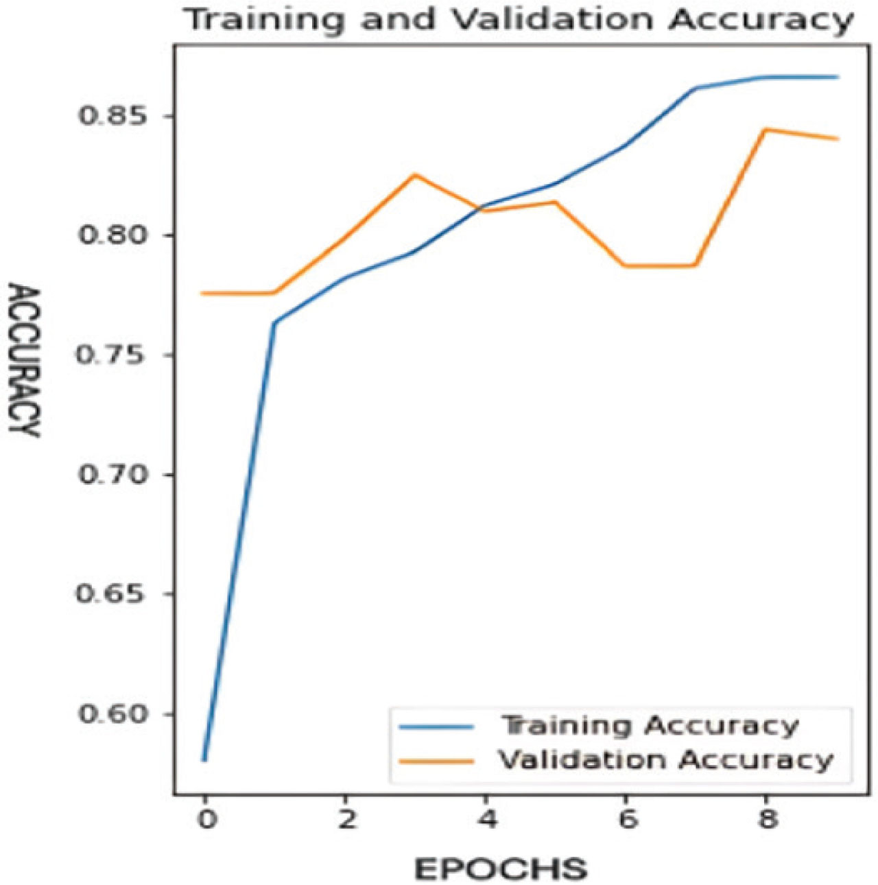
Figure 16:
Training and validation accuracy graph for four-layer CNN model without BN and dropout layers. BN, batch normalization.
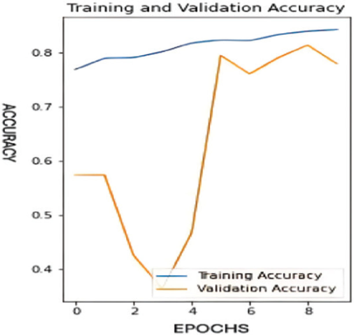
Figure 17:
Training and validation accuracy graph for four-layer CNN model with BN and dropout layers. BN, batch normalization.
Table 4 tabulates the four-layer model results, indicating that the model with BN and dropouts has encountered the problem of data leakage, and hence, there is a deterioration in all the performance metrics. This research study aims at analyzing and developing a simple yet high-performance model for medium sized dataset. Figures 18 and 19 show the confusion matrix for the four-layer CNN models.
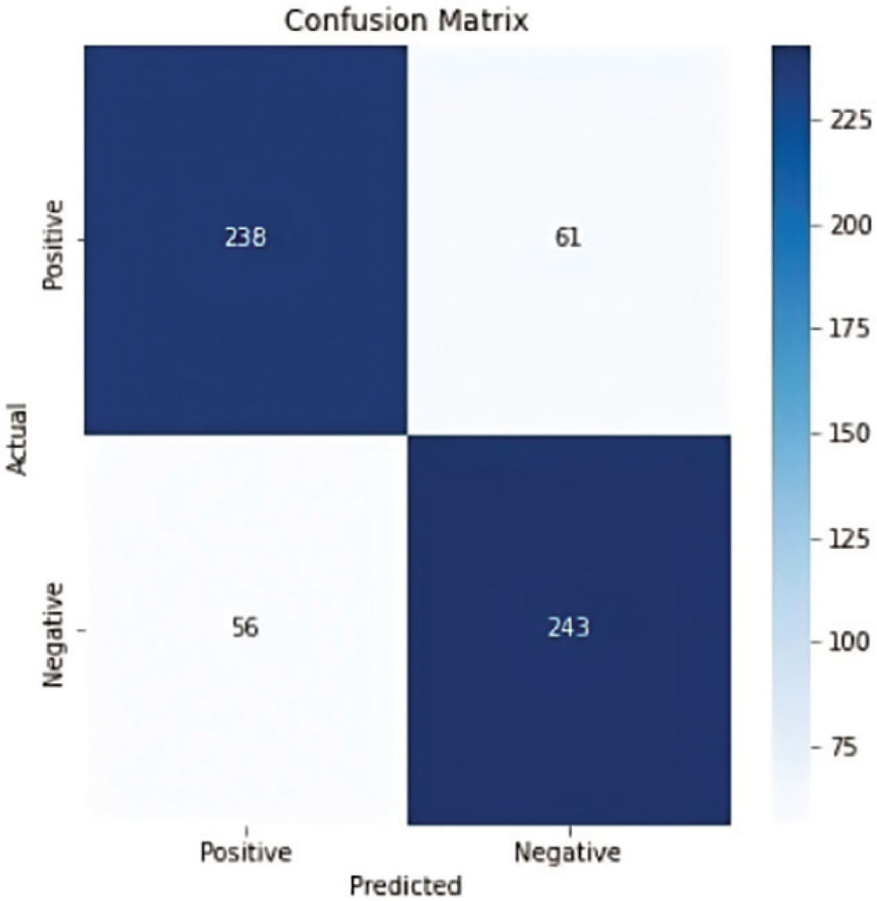
Figure 18:
Confusion matrix for CNN model without BN and dropout layers. BN, batch normalization.
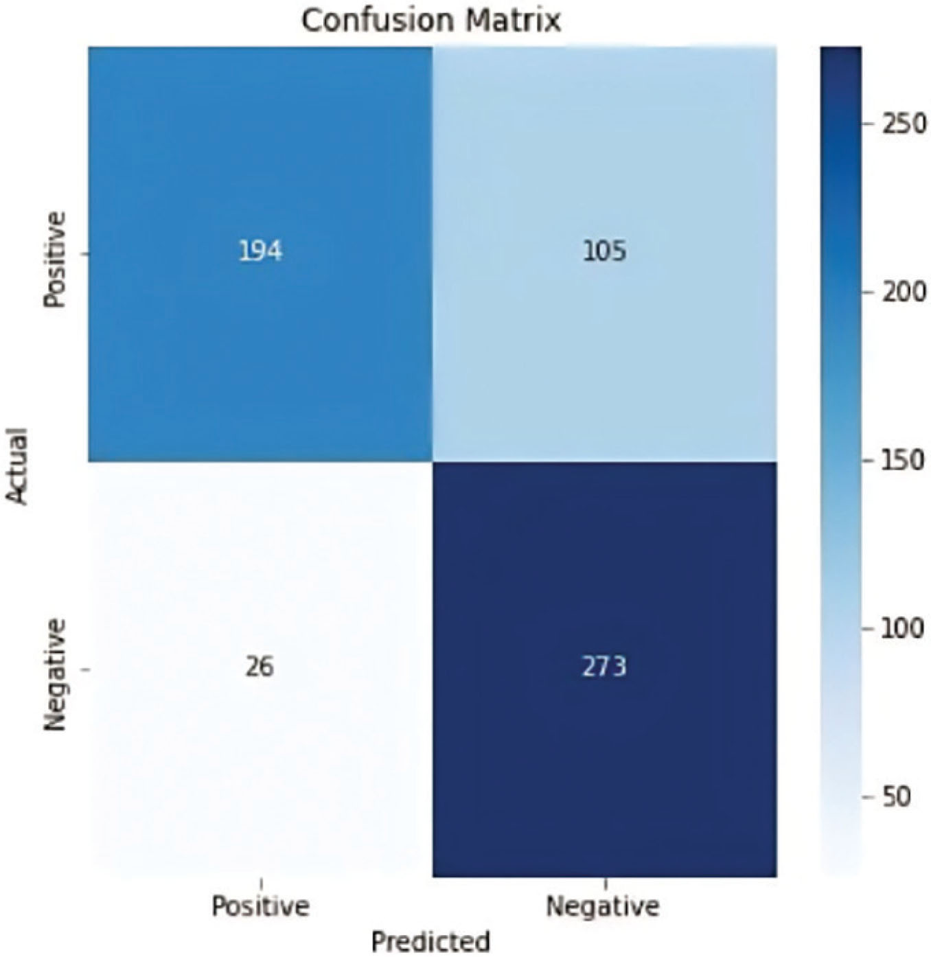
Figure 19:
Confusion matrix for CNN model with BN and dropout layers. BN, batch normalization.
VII. Comparative Study with Ensemble Classifiers
Feature extraction is a crucial preprocessing phase for any classifier to improve model performance. Extracting the most deterministic features leads to identifying the vital features that classify the images, which in turn aids in disease diagnosis and the patient treatment prognosis. The features affect computational efficiency based on the chosen classifier models. The features extracted from images are based on the visual, brightness, and texture. The images are generally analyzed in terms of the spatial or frequency domain. The frequency distribution of the color pixels in the image is extracted and termed as the frequency domain features of the image. These spatial and frequency domain features of any image are an excellent methodology for content-based retrieval of images and image analysis [38]. The visual features include HSV features, luminance, shape, and texture. The RGB color space is converted into a color space that demarcates the chrominance from luminance. The size of the lesion is a vital biomarker to distinguish cancerous cells. If the size of lesion is more than 6 mm, then the risk of lesion being malignant is higher [39]. The features such as convex area and solidity, are also significant biomarkers for cancer detection. Breast cancer detection from the mammogram image classification extracts texture features based on co-occurrence matrices [40]. The texture features are extracted with the color co-occurrence matrix (CLCM). CLCM is a matrix that defines the probability of occurrence of a similar pattern of pixels in the immediate neighborhood [41]. The RGB channels are separated and then for each channel, the GLCM is calculated to get CLCM [42]. The feature vector is extracted by computing Contrast, Correlation, Energy, and Homogeneity features for different combinations of the channels. The spatial relationship refers to the relative positions, sizes, and orientations of features of ROI in the image. This can be extracted by contour analysis, a method to analyze the spatial relationships of the objects in the image based on the positions, sizes, and orientations of these contours. To extract HSV features, the image is converted from RGB to HSV. The formula for HSV is given as Eqs. (18)–(20) [43].
The R, G, and B are red, green, and blue intensity values of the image. The feature vector is extracted from three combinations of color spaces. For an image Img represented in RGB color space, FVClcm is the feature vector for CLCM defined as Eq. (21).
The CLCM estimation for red channels, green channels, and blue channels is given in equation set of Eq. (22).
The shape features of skin lesions are one of the vital features to differentiate benign from malignant by medical examination. The shape of the affected region clearly depicts whether the lesion is malignant or benign. The features area, perimeter, and convexity are included in the feature set as shape features. The shape features of skin lesions are one of the vital features to differentiate benign from malignant by medical examination. The feature set is constructed from the extracted features. Table 5 shows the features included in constructing the dataset for the skin images.
Table 5:
Feature set extracted from the melanoma images
| Features | Feature set |
|---|---|
| Brightness Features | Luminance for LAB and YCBCR |
| HSV features | Hue, saturation, and value |
| Shape features | Area, perimeter, circularity, eccentricity, convex area, solidity, equivalent diameter |
| Texture features | Contrast, correlation, energy, homogeneity |
| Spatial features | Contour detection |
The ML classifiers use feature set acquired in the feature extraction stage to classify the skin lesion patterns. The common ML algorithms include SVM, Logistic Regression, k-nearest neighbor, and ensemble methods. The ensemble methods show improved classification performance compared to the single classifiers due to their robustness in discovering the data patterns. The weak learners in the ensemble classifier learn the relationship between the deterministic feature set and the response variables. Multiple base learners give multiple classification results for the same test data, which is resolved by the voting scheme. The conflicts in the multiple base learner predictions are solved by computing the average of the predicted values by each base learner. The common ensemble methods include Random Forest and AdaBoost [44]. Random Forest ensemble method is a bagging method where the sample data input for weak learner classifier is selected from the dataset by random sampling with replacement method. Random sampling with replacement ensures that the data is not just selected by a single base learner but by multiple base learners to improve the performance of the model. The AdaBoost method creates multiple stumps or small decision trees for each feature in the dataset. Based on the misclassification of the data samples by the stumps, the sample weights are updated to provide higher priority to the misclassified samples. The strength of ensemble method is reducing the chances of model overfitting. The model strives to attain a trade-off maintained between the bias and variance. Table 6 shows the experimental results of ML classifiers.
Table 6:
Experimental results of comparative study
| Classifiers | Precision | Recall rate | F1-score | Accuracy | |||
|---|---|---|---|---|---|---|---|
| B | M | B | M | B | M | ||
| SVM | 64 | 76 | 90 | 40 | 75 | 52 | 67 |
| LR | 64 | 73 | 88 | 40 | 74 | 52 | 66 |
| Desc tree | 78 | 74 | 78 | 74 | 78 | 74 | 76 |
| AdaBoost | 82 | 78 | 81 | 79 | 82 | 79 | 81 |
| Gradient boost | 83 | 77 | 81 | 81 | 83 | 80 | 81 |
| Random forest | 86 | 82 | 85 | 84 | 86 | 83 | 84 |
Figures 20–25 show the confusion matrix for the melanoma diagnosis with different classifiers. SVM is a very primitive ML algorithm, the performance is poor compared to all the other classifiers. Logistic regression performs poorly when there is no linear relationship between the feature variable and the response variable. Multicollinearity in the noisy dataset affects the model performance in LR. Decision tree overfits for noisy data, leading to poor performance. Data fragmentation affects the model performance and the classifier performance for this dataset is poor. Random Forest algorithm is robust with numerical data with outliers. In Random Forest, the decision trees are constructed independently and hence the order in which trees are constructed has no significant impact on the performance of the model. Whereas the order of stumps built in the AdaBoost classifier model affects the performance. The experimental results indicate that feature scaling is not mandatory for good performance of the Random Forest ensemble classifier. A high F1-score ensures that the model is sensitive to identifying all instances of positive class and there is a lesser number of false negative counts in the predictions. Figures 26–31 exhibits the ROC of SVM, LR. Decision tree, AdaBoost, Gradient Boost, and Random Forest.
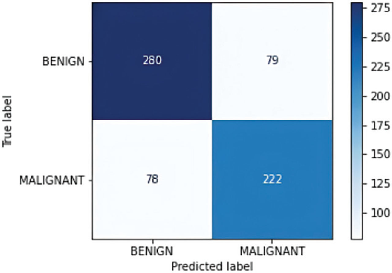
Figure 20:
Confusion matrix for SVM classifier.
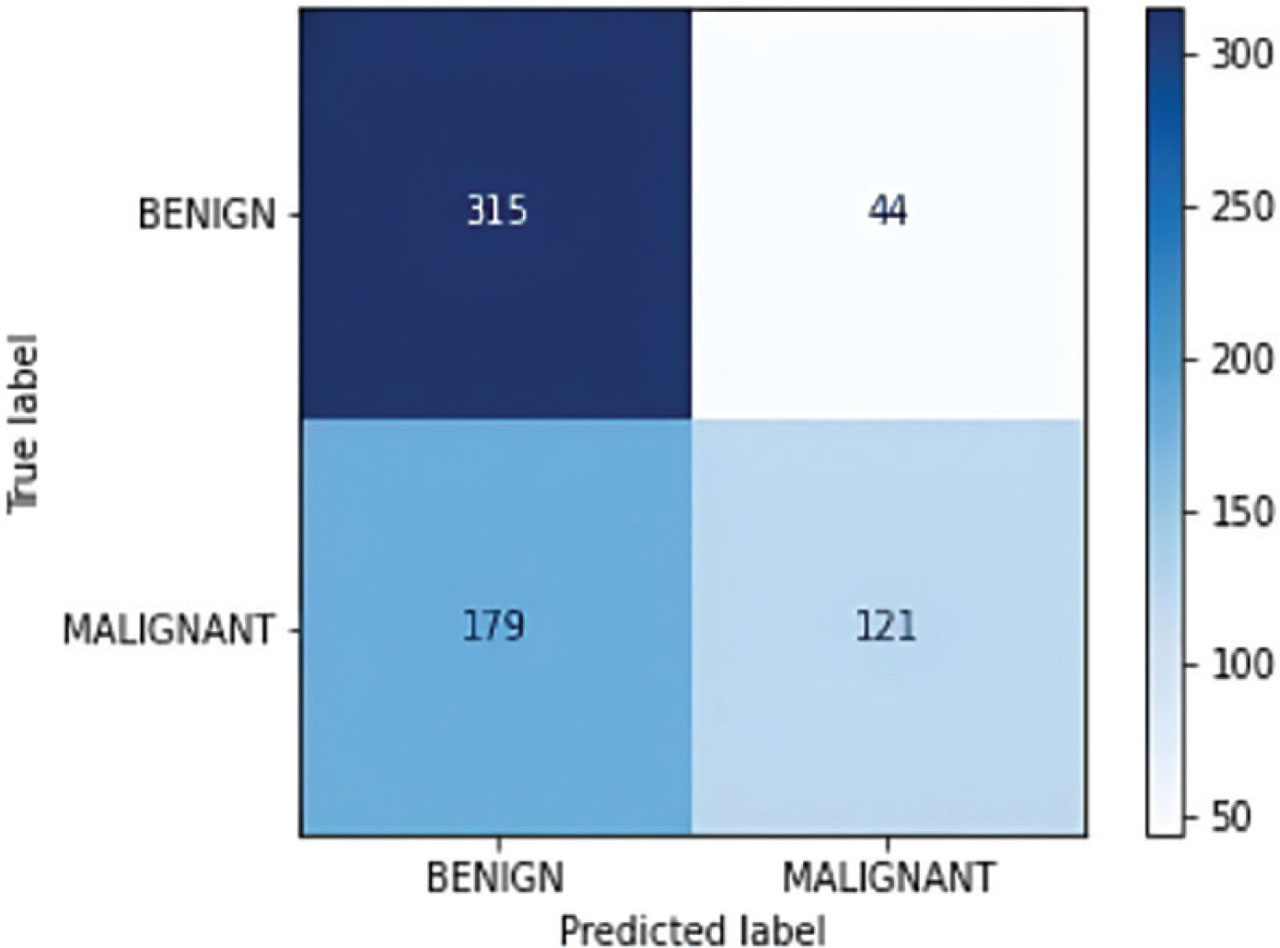
Figure 21:
Confusion matrix for logistic regression as classifier.
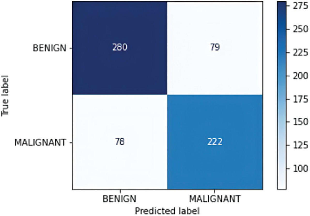
Figure 22:
Confusion matrix for decision tree as classifier.
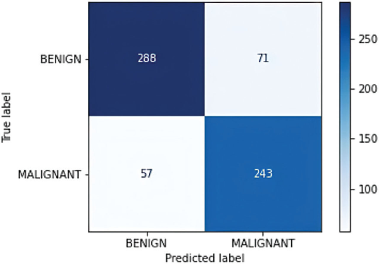
Figure 23:
Confusion matrix for AdaBoost as classifier.
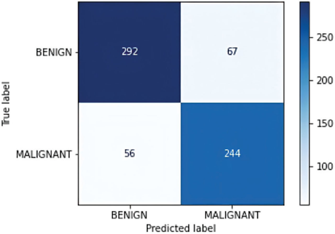
Figure 24:
Confusion matrix for gradient boosting as classifier.
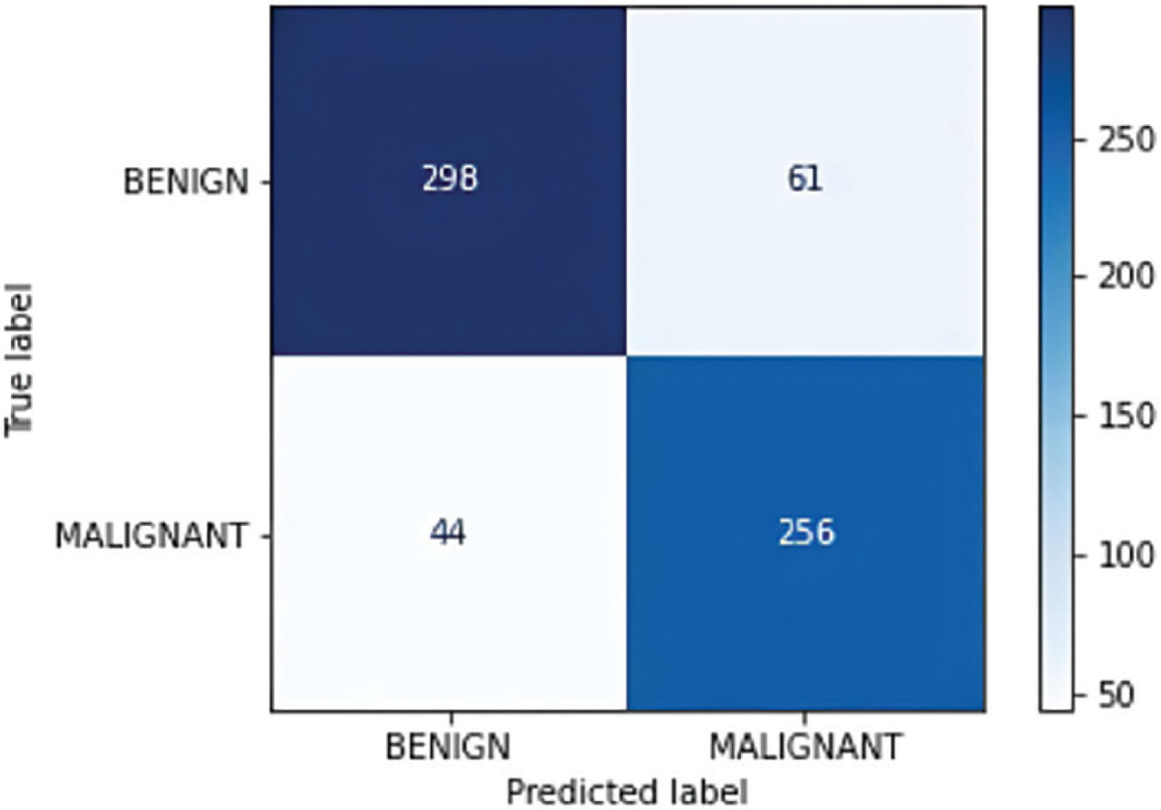
Figure 25:
Confusion matrix for random forest as classifier.
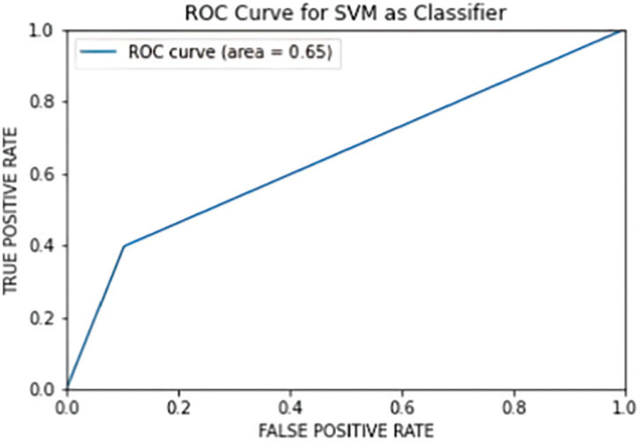
Figure 26:
ROC curve for SVM as classifier.
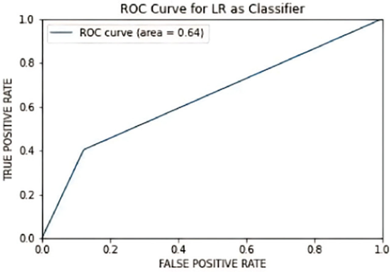
Figure 27:
ROC curve for LR as classifier.
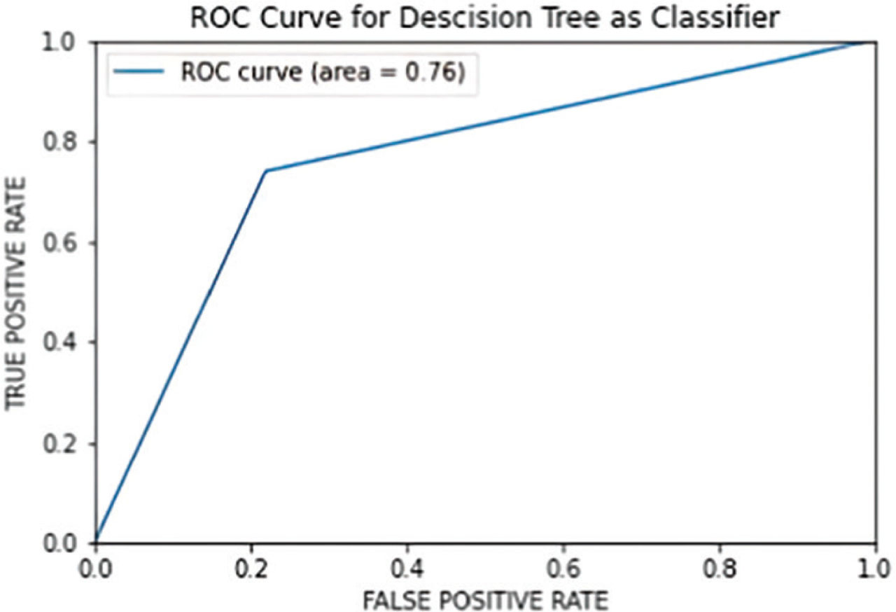
Figure 28:
ROC curve for decision tree as a classifier.
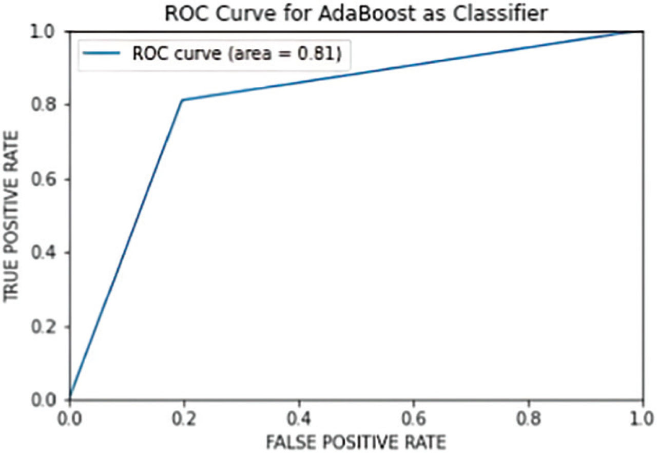
Figure 29:
ROC curve for AdaBoost as classifier.
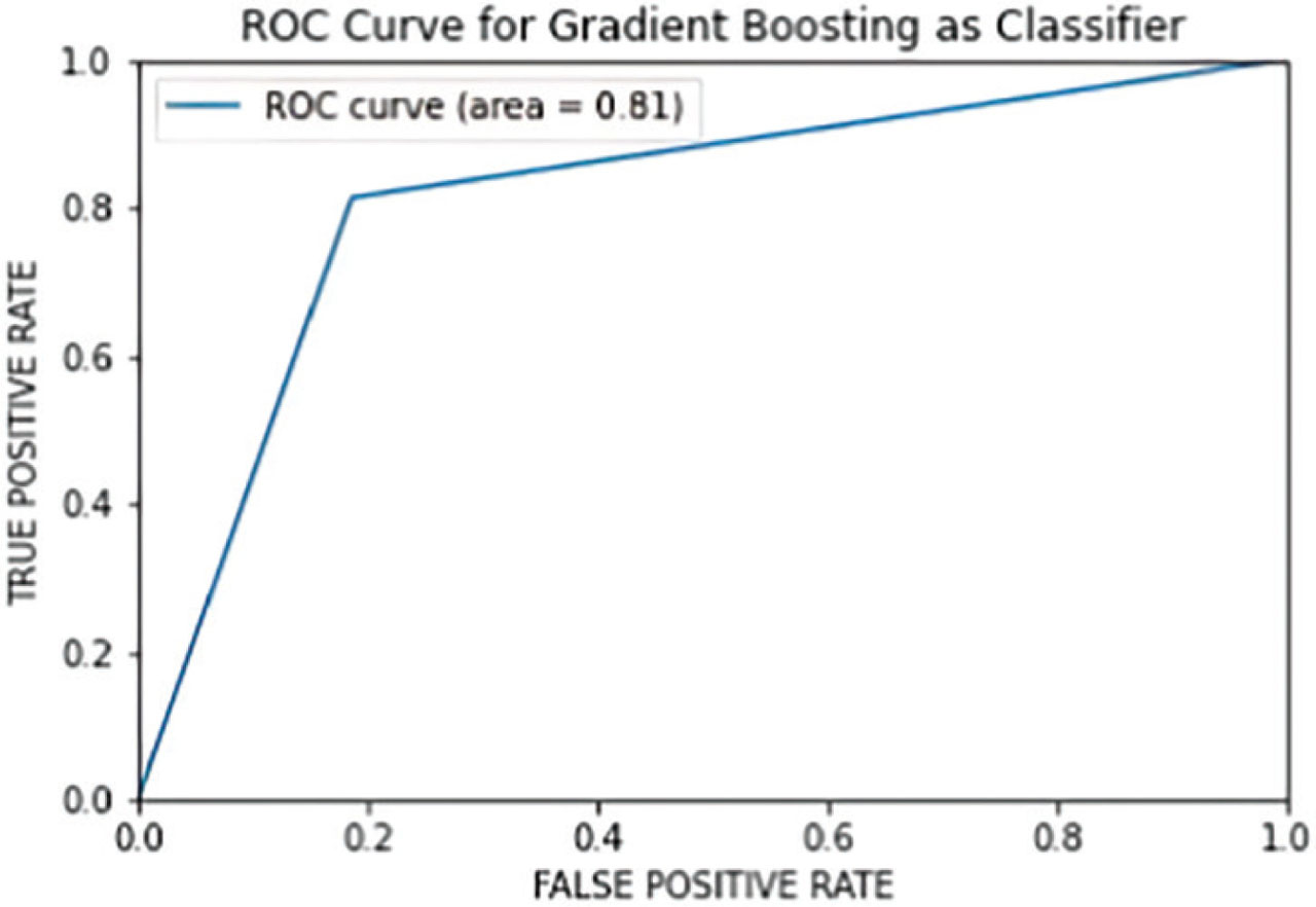
Figure 30:
ROC curve for gradient boosting as classifier.
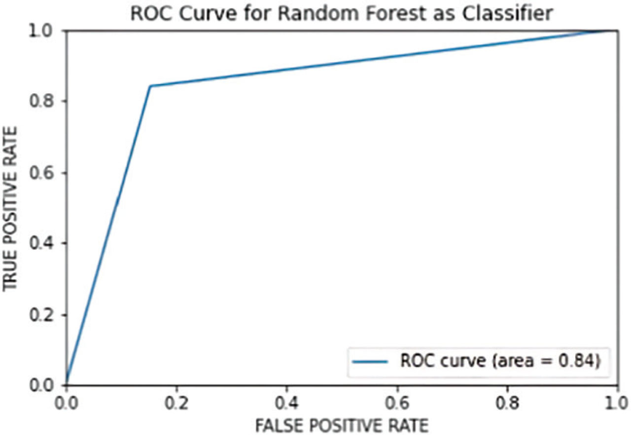
Figure 31:
ROC curve for random forest ensemble classifier.
Table 7 lists the state-of-the-art methodologies. The advantages of using a medium-sized dataset are rapid experimentation and prototyping with different architectures and hyperparameters. The risk of overfitting can be managed in medium-sized datasets well compared to larger ones. A medium-sized dataset balances the necessary data for learning the patterns without exhibiting complexity.
Table 7:
State-of-the-art methodologies for skin cancer diagnosis
| Study | Dataset | Skin Cancer | Technique | Accuracy (%) |
|---|---|---|---|---|
| I.S. Ali [8] | ISIC 2018 | a, b, c, e, f, h | PGAN | 70.1 |
| R.A. Mehr [10] | ISIC 2019 PAD-UFES-20 | a,b,e | Inception-ResNet-v2 CNN | 94.5±0.9 |
| AQ. Usca [11] | MSCD10000 | a | AlexNet CNN | 91.30 |
| N.M Mahmoud [16] | PH2 | a, b | ANN | 94 |
[i] (a) Melanoma; (b) Melanocytic nevus; (c) Basal cell carcinoma; (d) Benign keratosis; (e) Actinic keratosis; (f) Intraepithelial carcinoma; (g) Dermatofibroma; (h) Vascular lesions; (i) Benign melanocytic lesions; (j) Malignant and pre-malignant keratinocyte carcinoma; (k) Dermatofibroma; (l) Nevus pigmentosus; (m) Squamous cell carcinoma.
VIII. Challenges and Future Work
Future work includes conducting research study on a larger dataset for melanoma diagnosis. Availability of dataset is the main hurdle faced as it involves ethical issues. The future work also includes integrating federated ML in melanoma diagnosis. This concept focuses on a new perspective of training ML models on versatile data. Federated ML allows multiple model developers to train the model on their specific data and share the fine-tuned parameters to the centralized repository. On receiving significant data from the different models, the central aggregator will develop a more generalized model for the specific application. Federated learning systems face challenges like heterogeneous dataset, security issues, communication, and computation cost [45]. Computation costs can be reduced by selecting a subset of clients to share the model for training. Scalable aggregation algorithms reduce the communication and computation cost considerably. Federated learning can be adopted for challenges like medical image processing by data sharing. The advantage of adopting federated learning for similar challenges would be versatile data availability and reduced computation cost. The data collected for a particular group of users, considering their age, occupation, and domain for each individual model can enhance the global model. The multiple model parameters communicated to the central server develop a fine-tuned generalized model for a wider audience. The challenge faced will be data privacy while sharing the medical images. The challenges related to the proposed model being used in real-time environment are also worth discussing. The public dataset must include images of individuals from different demographic regions with versatile skin tones at different stages of melanoma for real time environment. Deploying this model in a resource-constrained environment is another challenge. It can be overcome by lightweight architectures on edge devices. Using them on a variety of devices from medical equipment to smart phones poses a challenge in real time environment. Strong testing methodologies can eliminate this concern. Confidentiality of patient data is an issue of concern. The patient record that includes sensitive information such as patient images should be protected throughout the development of the model. Strong encryption methods should be adopted while storage and transmission of these images. There should be transparency between the clinicians and patients in usage of data and how the decisions are made. This gives more clarity on the accountability of the decisions made by clinicians. The fact that AI is just an assistive tool to the clinicians and occurrence of false positives is inevitable should be made clear to the patients as a part of ethical consideration.
The scenario of scalability of the proposed system to clinical applications for larger datasets is discussed in this section. ESRGAN clearly improves image resolution in the pre-processing phase, but the time complexity intensifies with an increase in dataset size. The scalability can be handled efficiently through parallel ESRGAN inference on GPUs, batched processing, and offline caching of enhanced images prior to CNN training. The increase in the training time of the deep learning models ESRGAN and CNN can be mitigated by distributed training frameworks. High storage requirement is another issue raised due to scalability.
The advantage of scalability is improved performance of CNN due to large diverse datasets. CNN extracts more generalized features from the diverse skin melanoma images. CNN inherently scale more efficiently with larger datasets, exhibiting improved generalization performance due to versatile lesion availability and reduced overfitting issues. Model bias is reduced largely with scalability to larger datasets. Though the downsides of scalability are identified as time complexity and storage issues, the benefits are improved performance, reduced model bias, more generalization and wide use in clinical scenarios. The framework remains scalable for clinical deployment, as both ESRGAN and CNN can be executed on cloud-based GPU clusters, supporting high-throughput screening of dermatology images. This ensures that the model can handle large datasets without degradation in performance.
IX. Conclusion
The main goal of the proposed melanoma diagnosis model is to improve diagnostic accuracy and provide treatment to the patients at an early stage. This is an aid to the dermatologist to provide a second opinion on the case and to speed up the decision-making process. Such a diagnosis system can provide care for patients in remote areas with not many medical facilities and enhance telemedicine and remote diagnostics. This tool can empower general physicians to refer to dermatologists. This may avoid unnecessary referrals for diagnosing the risk of melanoma. Such AI models create awareness among patients regarding melanoma and help in their early diagnosis. This novel framework developed for melanoma diagnosis leverages the advantages of ESRGAN, density clustering, and deep learning techniques to show improved accuracy compared to the state-of-the-art methodology. ESRGAN is well known for generating a set of novel super-resolution images that positively impact the performance of the classifier model. The study compares a naïve CNN model performance with the custom-built CNN model for a dataset of ESRGAN-generated super-resolution images. The significant finding of this research work asserts that pre-processing and further image enhancement show remarkable improvement in the model performance compared to the model without image enhancement phase. This proposed unique model can discover intricate patterns in the image and classify them accurately compared to the discussed state-of-the-art framework. The disadvantage of the deep learning techniques is the computational cost that demands high-end infrastructure. The deep learning approach is strongly recommended for medical imaging, as false predictions are negligible when the framework is well designed.
X. Recommendations
Artificial intelligence model performance relies on learning algorithms and quality of real-world data. Real-time data, with its outliers, missing values, and ambiguity, requires preprocessing and feature reduction before classification or prediction. To be precise, traditional ML algorithms demand feature engineering process before the classification phase. Hence, this research study adopts deep learning technique of CNN for classification. The artificial neural network ESRGAN was adopted for generations of high-resolution images for the deep learning model. ESRGAN leverages GAN technology to produce realistic textures in high-frequency regions such as edges and fine patterns, surpassing methods like VDSR or Bicubic that struggle to deal with such fine details. ESRGAN introduces the RRDB architecture, which improves information flow and reduces the risk of gradient vanishing, enabling improved learning of intricate details. The finding revealed that image enhancement with ESRGAN generates high-resolution images of ground truth images and this is experimentally proved by recording the PSNR and SSIM metrics for the images. DBCESp has improved the performance of a simple CNN customized configuration. The performance of the proposed model is at par with a complex deep learning neural network model, which has high computational complexity. There are a couple of competent segmentation techniques for versatile medical images, and finding the best technique among them can be invariably challenging. The disadvantage of density-based clustering is converging toward the local optima, and this problem is addressed with Salp optimization algorithm. An extensive comparative study of ML classifiers to the ensemble methods of AdaBoost and Random Forest is implemented and tabulated. In a traditional ML framework, feature extraction from segmented regions of the image is a far-reaching task. However, researchers strongly recommend feature selection to identify the most discriminating features correlated with the response variable in the dataset for traditional ML algorithms. Identifying the best feature extraction algorithm and selecting the optimum feature set contribute to model performance in any ML algorithm. The comparison study with DBCESp and ensemble classifier shows an accuracy of 85% for Random Forest and 81% for AdaBoost. The Random Forest algorithm performs better than the AdaBoost and gradient boosting algorithms for this dataset. The feature set extracted from the images is a numerical dataset with outliers and is better handled by the Random Forest classifier.
Acknowledgment
The authors extend their appreciation to Prince Sattam bin Abdulaziz University for funding their research work through project number (PSAU/2025/R).
Notes
[6] Ethical statement
This study does not contain any studies with human or animal subjects performed by any of the authors.
[7] Conflicts of interest Conflicts of interest
The authors declare that they have no conflicts of interest in this work.
[8] Data availability statement
International Skin Imaging Collaboration. Available online: https://www.isic-archive.com/ (Accessed on Nov. 20, 2023).