
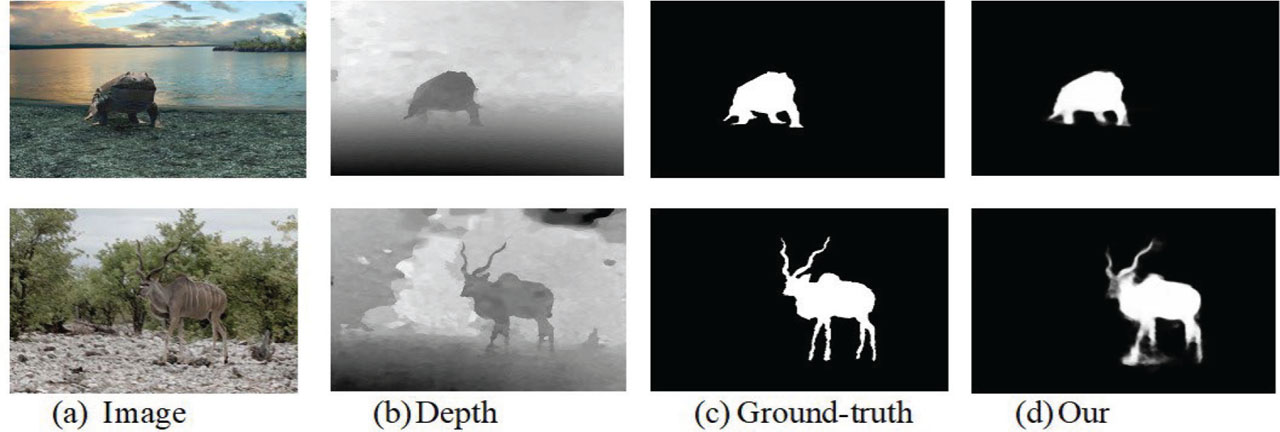
Figure 1:
The demonstration of multi-horizon-attention and feature optimization using muti-scaled, multi-resolution, multi-stage color, depth, and common modality-based features. (A) Image. (B) Depth. (C) Ground-truth. (D) Our.
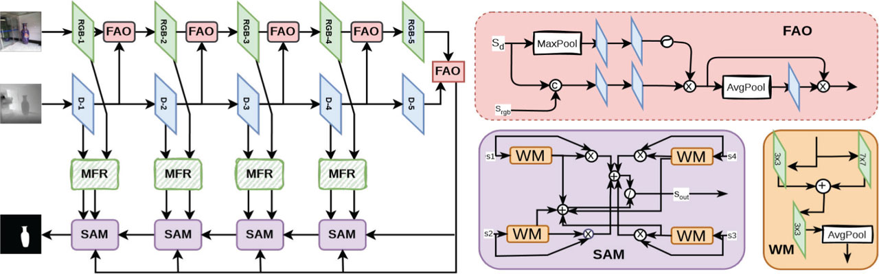
Figure 2:
The left part shows the architecture of the proposed model. First, the model extracts features from the RGB image and depth map. While extracting the complementary features, the RGB FAO. Then these cross-model features are fused in a MFR. Finally, the outputs of these MFR modules are fed to a SAM in four steps to obtain the final saliency map. FAO, feature aggregation and optimization; MFR, multi-horizon feature reconstruction; SAM, self-aggregation module.
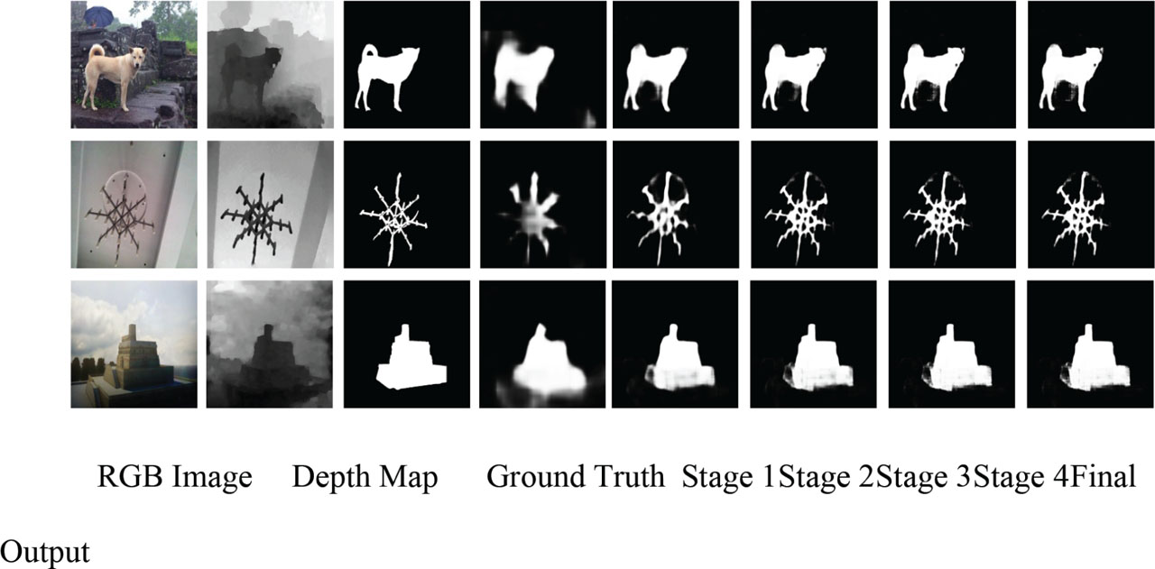
Figure 3:
Stage-wise optimization of extracted features has visualized the reconstruction of visual salient points in the low-depth images to predict the salient objects accurately.
Table 1:
The quantitative comparison of the proposed model on six benchmark RGBD datasets with four recent evaluation parameters.
| Date-Set | Metric | OUR | Improving [53] | CATNet [54] | FCN [37] | AirSod [25] | MAD [55] | DCMF [56] | GCFNET [22] | HIFN [50] | CAS-GNN [29] | cmMS [33] | CoNet [51] | D3Net [20] | CPFP [15] | TANet [57] | PCFNET [52] | CTMF [27] | AFNet [26] | DF [13] |
|---|---|---|---|---|---|---|---|---|---|---|---|---|---|---|---|---|---|---|---|---|
| NJUD [6] | Fβ↑ | 0.945 | 0.940 | 0.929 | 0.918 | 0.918 | 0.903 | 0.888 | 0.915 | 0.915 | 0.893 | 0.914 | 0.872 | 0.900 | 0.877 | 0.874 | 0.872 | 0.845 | 0.775 | 0.804 |
| Sα↑ | 0.941 | 0.926 | 0.937 | 0.918 | 0.908 | 0.921 | 0.913 | 0.914 | 0.912 | 0.911 | 0.900 | 0.894 | 0.900 | 0.879 | 0.878 | 0.877 | 0.849 | 0.772 | 0.763 | |
| Eψ↑ | 0.969 | 0.959 | 0.933 | 0.953 | 0.944 | 0.930 | 0.925 | 0.947 | 0.944 | 0.922 | 0.914 | 0.912 | 0.950 | 0.926 | 0.925 | 0.924 | 0.913 | 0.853 | 0.864 | |
| MAE↓ | 0.024 | 0.026 | 0.025 | 0.039 | 0.034 | 0.037 | 0.043 | 0.038 | 0.038 | 0.036 | 0.044 | 0.047 | 0.041 | 0.053 | 0.060 | 0.059 | 0.085 | 0.100 | 0.141 | |
| NLPR [46] | Fβ↑ | 0.928 | 0.934 | 0.916 | 0.911 | 0.923 | 0.901 | 0.875 | 0.907 | 0.915 | 0.888 | 0.913 | 0.850 | 0.897 | 0.867 | 0.863 | 0.841 | 0.825 | 0.771 | 0.778 |
| Sα↑ | 0.949 | 0.932 | 0.939 | 0.924 | 0.908 | 0.933 | 0.922 | 0.919 | 0.924 | 0.919 | 0.899 | 0.907 | 0.912 | 0.888 | 0.886 | 0.874 | 0.860 | 0.799 | 0.802 | |
| Eψ↑ | 0.966 | 0.966 | 0.968 | 0.960 | 0.963 | 0.955 | 0.940 | 0.953 | 0.960 | 0.951 | 0.945 | 0.936 | 0.953 | 0.932 | 0.941 | 0.925 | 0.929 | 0.879 | 0.880 | |
| MAE↓ | 0.019 | 0.019 | 0.018 | 0.024 | 0.039 | 0.022 | 0.029 | 0.025 | 0.924 | 0.025 | 0.027 | 0.031 | 0.030 | 0.036 | 0.041 | 0.044 | 0.056 | 0.058 | 0.085 | |
| STEREO [47] | Fβ↑ | 0.945 | 0.933 | 0.902 | 0.906 | 0.900 | 0.892 | 0.872 | 0.900 | 0.906 | 0.876 | 0.908 | 0.885 | 0.891 | 0.871 | 0.861 | 0.860 | 0.831 | 0.823 | 0.757 |
| Sα↑ | 0.933 | 0.922 | 0.925 | 0.906 | 0.895 | 0.910 | 0.903 | 0.899 | 0.907 | 0.899 | 0.889 | 0.908 | 0.899 | 0.879 | 0.874 | 0.875 | 0.848 | 0.825 | 0.757 | |
| Eψ↑ | 0.967 | 0.953 | 0.935 | 0.947 | 0.939 | 0.939 | 0.930 | 0.940 | 0.944 | 0.929 | 0.922 | 0.922 | 0.938 | 0.925 | 0.923 | 0.925 | 0.912 | 0.887 | 0.847 | |
| MAE↓ | 0.031 | 0.026 | 0.030 | 0.032 | 0.043 | 0.037 | 0.043 | 0.040 | 0.040 | 0.039 | 0.042 | 0.041 | 0.046 | 0.051 | 0.060 | 0.064 | 0.086 | 0.075 | 0.141 | |
| SSD [48] | Fβ↑ | 0.889 | 0.861 | - | - | - | 0.850 | - | - | 0.870 | 0.840 | 0.865 | 0.806 | 0.834 | 0.766 | 0.810 | 0.807 | 0.729 | 0.687 | 0.735 |
| Sα↑ | 0.887 | 0.871 | - | - | - | 0.872 | - | - | 0.875 | 0.872 | 0.874 | 0.853 | 0.857 | 0.807 | 0.839 | 0.841 | 0.776 | 0.711 | 0.747 | |
| Eψ↑ | 0.940 | 0.917 | - | - | - | 0.907 | - | - | 0.917 | 0.915 | 0.911 | 0.896 | 0.910 | 0.852 | 0.897 | 0.894 | 0.865 | 0.807 | 0.828 | |
| MAE↓ | 0.042 | 0.045 | - | - | - | 0.045 | - | - | 0.045 | 0.047 | 0.052 | 0.059 | 0.058 | 0.082 | 0.063 | 0.062 | 0.099 | 0.118 | 0.142 | |
| LFSD [49] | Fβ↑ | 0.919 | 0.857 | 0.884 | 0.876 | - | 0.862 | 0.771 | 0.771 | 0.849 | 0.832 | 0.888 | 0.848 | 0.810 | 0.826 | 0.796 | 0.775 | 0.787 | 0.744 | 0.813 |
| Sα↑ | 0.909 | 0.821 | 0.894 | 0.875 | - | 0.867 | 0.879 | 0.846 | 0.845 | 0.846 | 0.846 | 0.862 | 0.825 | 0.828 | 0.801 | 0.786 | 0.788 | 0.738 | 0.783 | |
| Eψ↑ | 0.930 | 0.849 | 0.908 | 0.913 | - | 0.901 | 0.842 | 0.883 | 0.907 | 0.877 | 0.891 | 0.897 | 0.862 | 0.872 | 0.847 | 0.827 | 0.857 | 0.815 | 0.857 | |
| MAE↓ | 0.041 | 0.096 | 0.051 | 0.061 | - | 0.059 | 0.068 | 0.079 | 0.070 | 0.074 | 0.72 | 0.071 | 0.095 | 0.088 | 0.111 | 0.119 | 0.127 | 0.133 | 0.145 | |
| DUT-RGBD [5] | Fβ↑ | 0.960 | 0.859 | 0.951 | 0.931 | 0.920 | - | 0.928 | 0.923 | 0.913 | 0.912 | 0.932 | 0.908 | 0.867 | 0.795 | 0.790 | 0.771 | 0.823 | 0.659 | 0.744 |
| Sα↑ | 0.957 | 0.841 | 0.953 | 0.924 | 0.891 | - | 0.920 | 0.918 | 0.902 | 0.891 | 0.885 | 0.918 | 0.882 | 0.818 | 0.808 | 0.801 | 0.831 | 0.762 | 0.705 | |
| Eψ↑ | 0.977 | 0.879 | 0.971 | 0.956 | 0.946 | - | 0.950 | 0.951 | 0.929 | 0.932 | 0.940 | 0.941 | 0.889 | 0.859 | 0.861 | 0.856 | 0.899 | 0.796 | 0.823 | |
| MAE↓ | 0.020 | 0.071 | 0.020 | 0.032 | 0.048 | - | 0.043 | 0.040 | 0.041 | 0.043 | 0.036 | 0.034 | 0.061 | 0.076 | 0.093 | 0.100 | 0.097 | 0.122 | 0.145 |
Table 2:
Illustration of the contribution of optimization of each component of the proposed model.
| Setting | STEREO [47] | NJU2K [6] | LFSD [49] | |||||||||||||
|---|---|---|---|---|---|---|---|---|---|---|---|---|---|---|---|---|
| BASE MODEL | Low-depthissues | OUR | MFR | SAM | Fβ↑ | Sα↑ | Eψ↑ | MAE↓ | Fβ↑ | Sα↑ | Eψ↑ | MAE↓ | Fβ↑ | Sα↑ | Eψ↑ | MAE↓ |
| ✓ | 0.8038 | 0.8064 | 0.8572 | 0.0894 | 0.7559 | 0.7766 | 0.7703 | 0.1003 | 0.7095 | 0.7105 | 0.7090 | 0.1963 | ||||
| ✓ | ✓ | 0.8152 | 0.8334 | 0.8442 | 0.0840 | 0.7889 | 0.8690 | 0.8088 | 0.0900 | 0.7245 | 0.7505 | 0.7590 | 0.1083 | |||
| ✓ | ✓ | ✓ | 0.8481 | 0.8452 | 0.8555 | 0.0752 | 0.8245 | 0.8489 | 0.8505 | 0.0762 | 0.8335 | 0.8452 | 0.8580 | 0.0882 | ||
| ✓ | ✓ | ✓ | ✓ | 0.8582 | 0.8609 | 0.8781 | 0.0651 | 0.8772 | 0.8778 | 0.8780 | 0.0610 | 0.8676 | 0.8590 | 0.8775 | 0.0790 | |
| ✓ | ✓ | ✓ | ✓ | ✓ | 0.9456 | 0.9334 | 0.9674 | 0.0310 | 0.9456 | 0.9414 | 0.9698 | 0.0245 | 0.9197 | 0.9097 | 0.9370 | 0.0411 |
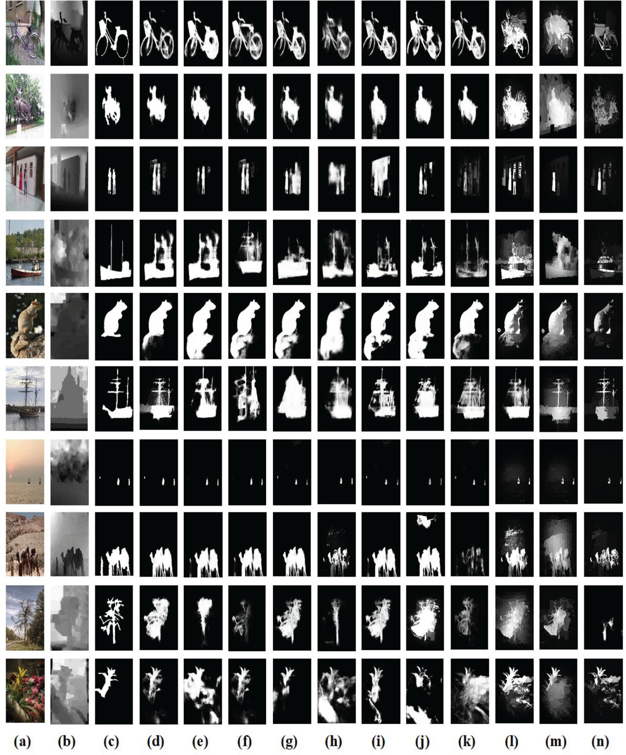
Figure 4:
The saliency maps is shown here for the visual demonstration (A) input RGB image, (B) depth image, (C) GT image, (D) OUR, (E) HAIN, (F) CAS−GNN, (G) cmMS, (H) CoNet, (I) D3NET, (J) CPSF, (K) TANet, (L) PCFNET, (M) CTMFR, and (N) AFNet of proposed model. GT, ground truth.
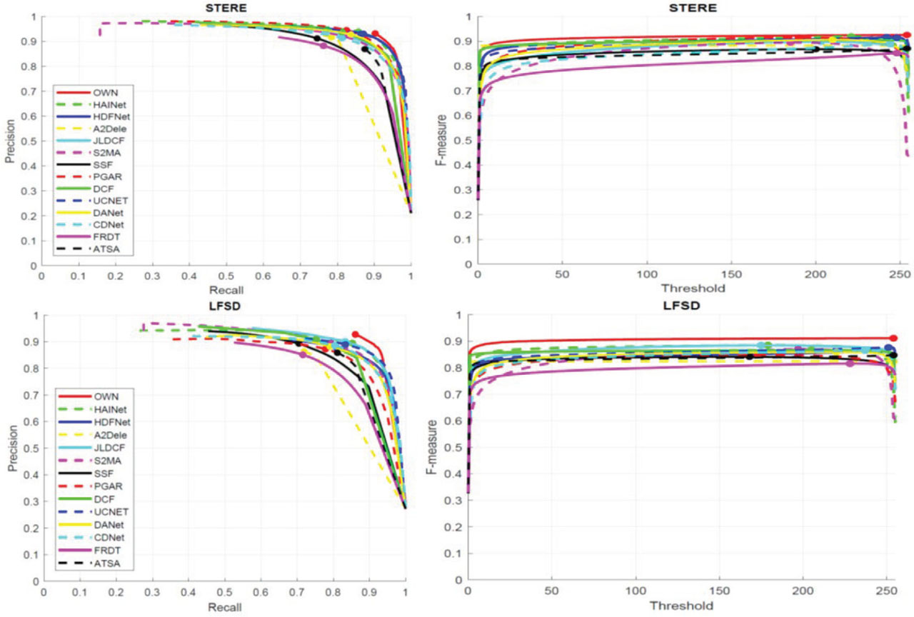
Figure 5:
Comparison of our proposed model with recent models with (A) PR-curve (B) F-measure (vertical axis (thresholds) and horizontal axis) datasets (1) STERE (2) LFSD dataset, respectively.