
I. Introduction
Salient object detection (SOD) refers to the task of identifying prominent objects and regions in complex images, similar to the way humans identify them. Recently, SOD has attracted significant interest in the community and has become increasingly popular due to advances in depth sensing technologies. Hence, depth information is an essential parameter for detecting salient objects in low-depth images. SOD has appeared in pre-processing or as an integral part of many vision-related applications, such as semantic segmentation [1], object classification [2], video summarization [3], and content-based image editing [4].
In this paper, we propose a multi-horizon-attention mechanism, that is, feature aggregation and optimization (FAO)-based deep learning model that explores all possible features in a cascade-combine manner. The proposed model is based on a three-stream fusion network targeting non-complementary information in RGB and depth modalities, as purely color contrast-based features, depth contrast-based features, and regional color features, which are shown in Figure 1. The features in the two sub-networks are fused level-wise to extract complementary information between the two modalities and intra-complementary features between deep and shallow levels, as well as high-level contextual, semantic, structural, and spatial global features.
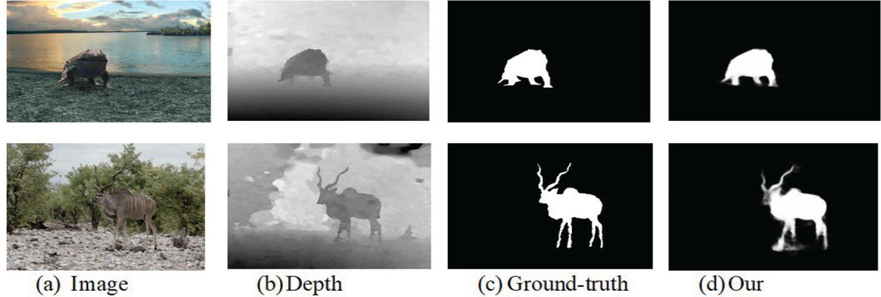
Figure 1:
The demonstration of multi-horizon-attention and feature optimization using muti-scaled, multi-resolution, multi-stage color, depth, and common modality-based features. (A) Image. (B) Depth. (C) Ground-truth. (D) Our.
Early approaches in RGB-D SOD [5,6,7,8,9,10,11,12] are based on low-level, handcrafted features in both modalities separately. These models perform poorly on complex and cluttered background images. They have limited performance with low-depth images. CNN-based shallow deep learning models [13] integrate both modalities in a much more generalized manner. Since then, several CNN-based models have been proposed with improved performance; however, there remains a wider scope for further improvements.
These models are classified according to their architecture into (1) single-stream models and (2) multi-stream models. CNN-based RGB-D SOD models started with a single stream network mainly [13,14,15,16,17,18]. DANet [19] fused the color and depth features to predict the final saliency. In a multi-stream network [13, 14], some features are computed traditionally, which are used to guide the single-stream networks to compute the saliency. Other models [16] use a late fusion strategy to predict saliency maps. PDNet [17] was proposed with a single stream based on multi-stage features which are fused through guidance from a subsidiary depth network. These models have limited efficiency in terms of fusion of the different modalities to predict the saliency correctly. Another proposed approach [19,20,21] has two separate streams dedicated to each modality, which extract high-level semantic features independently and then fuse them using a middle or late fusion. The low-depth issues are addressed recently [22,23,24,25] by proposing an enhanced fusion mechanism. The proposed model focuses on optimization of low-depth issues and proposes an efficient fusion mechanism to explore the optimal complementary features across the two modalities at different stages. For the above-mentioned challenges, our proposed model, feature optimization using a multi-horizon reconstruction module, makes the following contributions to improve the state-of-the-art fusion process.
The proposed model enhances stage-wise RGB, depth complementary features using multi-horizon feature reconstruction (MFR) mechanism in low-depth images.
In this paper, we propose a novel MFR module to enhance feature extraction from the two modalities, along with attention-based refinement of RGB data using composite backbone network.
We designed a FAO module to decode the encoded features from the fused stream in a hierarchical manner using self-attention weight.
The proposed model uses feature reconstruction to provide robust characteristics even in complex and cluttered backgrounds, demonstrated by using recent evaluation metrics with state-of-the-art methods.
The paper is organized into the following sections. Section II provides a detailed survey of related deep learning works in the domain. Section III describes the proposed method, and Section IV discusses the experimental setup while demonstrating the performance of the proposed model with other state-of-the-art methods. Section V describes the conclusion and future scope of the proposed model for further improvements.
II. Related Works
Initially, depth-based non-deep learning SOD models [5] were based on handcrafted features. The CNN-based discriminative features have been currently utilized for accurate prediction. The main focus of recent models is proposing efficient fusion processes with attention mechanisms to address low-depth issues. Recently, 3D saliency models have produced more accurate predictions based on an optimized fusion model.
The early fusion strategy [13, 18] exploited handcrafted features, while, the late fusion strategy [26, 27, 20] utilized full CNN features. Furthermore, it adopts some statistical models to fuse the computed saliency features. The cross-modality-based complementary features are a recent domain to optimize fusion strategy. In this middle-level fusion strategy [23, 24, 28,29,30,31] side-output or skip-connection-based features are used. The fusion process is based on using multi-scale features with cross-combination blocks.
The main feature extraction is studied and analyzed in the following two streams. The single-stream models [13, 15, 18, 24, 32] simultaneously extract the color and depth features. While in multi-stream models [28, 31, 33], modality-dependent features are extracted separately. For example, Zhao et al. [19] DANet used RGB and depth images collectively in a single encoder. These models do not separately emphasize the RGB and depth features. At the same time, in a multi-stream architecture, the two parallel encoders are used. These features are combined within a middle-level strategy to predict saliency. For example, [34] designed two-stream models and progressively fused the multi-level features from RGB and depth streams alternately by proposing a multi-scale residual block.
Nevertheless, these models do not improve the essential features and propagate the extraction of irrelevant saliency features in multi-stage encoders. Consequently, these models destroy border-region saliency. Furthermore, the aforementioned models are eradicating the salient regions, which are similar to background regions in complex scenarios.
Low-depth model: Recent models mainly focused on removing the low depth and occlusion-based depth issues by proposing attention to the depth modality to improve depth information. Encouraging performance has been achieved, yet leaving enormous scope for further improvements. Pang et al. [31] proposed a hierarchical dynamic filtering network (HDFN) to purify the cross-modality fusion features through a densely connected structure. Furthermore, several approaches such as [20, 34,35,36,37], AirSOD [22,23,24,25] used depth maps as auxiliary or complementary information to the RGB stream without using both streams as complementary to each other to solve the low-depth issues. Zhang et al. [38] introduced two-stream architectures, each for RGB and depth modality to enhance the complementary features. However, it failed to propagate the irrelevant saliency features during the encoding stages.
Most recent works on RGBD SOD have achieved promising results by improving the quality of raw depth information. Piao et al. [35] proposed a network by using depth information to improve RGB features by knowledge distillation. It reduced the depth-related information loss. Similarly, the feature calibrating and fusing network [37] used three modules to calibrate unreliable depth information and improve cross-modality information. Another recent model, AirSOD [25], was proposed to achieve long-range contextual and local Information from depth modalities to improve performance. These models achieved promising results by improving the influence of low-quality depth images. Nevertheless, the above models still fail to optimize both modalities to exploit the contextual, structural, and high-level semantic information due to the influence of inconsistent depth images.
Attention-based model: Recently, the regional and spatial disparity in saliency computation has been addressed by attention mechanisms. In this mechanism, different weights are computed to distinguish the various missing regions. Initially, the attention weight is mainly computed based on depth modality [15] and channel-wise attention weight [39]. These attention weights differentiate the appearance features. The structural and contextual weights have not yet been utilized. The self-attention, and nonlocal-based attention weights [40,41,42,43,44] compute a self-mutual attention map, which is mainly used in language modeling and other query-based applications. We formulate various attention models, such as channel-wise attention, spatial attention, and mutual attention, to enhance structural, contextual, and high-level localized semantic features while minimizing irrelevant features.
The above-mentioned limitations of existing contemporary SOD models are addressed by proposing the multi-horizon attention-based backbone network with a self-learning-based decoder. In this proposed model, the FAO model is used to enhance stage-wise high-level structural and semantic features by using low-level contextual information. The MFR module integrates the relevant features and minimizes the propagation of irrelevant features by using multiple attention mechanisms at multiple stages.
III. Proposed Model
a. Model overview
Our methodology follows a three-step process: (1) Feature Extraction, (2) MFR, (3) FAO. We use convolution layers from a VGG-16 network. It is pre-trained on the ImageNet dataset for feature extraction. The detailed architecture of individual components of our proposed model is shown in Figure 2.
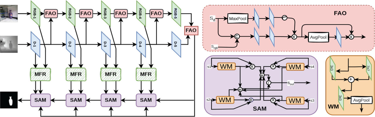
Figure 2:
The left part shows the architecture of the proposed model. First, the model extracts features from the RGB image and depth map. While extracting the complementary features, the RGB FAO. Then these cross-model features are fused in a MFR. Finally, the outputs of these MFR modules are fed to a SAM in four steps to obtain the final saliency map. FAO, feature aggregation and optimization; MFR, multi-horizon feature reconstruction; SAM, self-aggregation module.
b. Feature extraction
The RGB images and depth maps are fed into two separate networks, where we use the first four layers of the VGG network for feature extraction. After each layer in the RGB network, we optimize the extracted FAO module, which takes features from the depth and RGB networks as input.
c. Feature aggregation and optimization
Inside a FAO module, the depth maps are passed through a max-pooling layer followed by two convolutional layers of 3 × 3 and 7 × 7 which is shown in Figure 2. The obtained output is then passed into the softmax function to get the channel-wise attention weights. On the other hand, the and are concatenated, followed by two convolutions of 3 × 3 and 7 × 7 to obtain the mutual attention weights.
Then, we perform a matrix multiplication of the channel-wise attention weights and mutual attention weights to get . After taking an average pool, this is then fed to a 1 × 1 2D convolutional layer. We perform a matrix multiplication of the result with to obtain the combined attention weight . Finally, we perform an element-wise addition of the combined attention weights with and . This gives us , which can be mathematically stated as follows in Eq. (1):
d. MFR
The extracted optimized features are fused step-by-step using the MFR module. The outputs of the first four VGG layers in both sides of the architecture and are divided into four parts by applying 3 × 3 dilated convolutions parallelly to give and on RGB images and depth maps, respectively. For jth dilation rate can be given by 2j −1, where j can be between 1 and 4, both inclusive. To obtain the fused output for each dilated part can be described in Eq. (2):
The CCF of two features is given by the sum of two feature matrices and element-wise matrix multiplication of the two feature matrices. This can be mathematically stated as follows:
where ⊕ is the element-wise addition operator and ⊗ is the element-wise multiplication operator, which is defined in Eq. (3).Finally, we concatenate each of the for all j = 1–4 in Eq. (4), to receive the multi-horizon reconstruction fused features as follows:
Along with this, we also compute the CCF of and to get the multi-horizon complementary features for the current layer, which is defined in Eq. (5).
e. Self-aggregation module
Once we have the fused RGB and depth-optimized features, we aggregate these into individual saliency maps for each of the four pairs of fused features using a self-aggregation module (SAM). The enhanced output from the last VGG layer is treated as the input for all SAM modules, where we upsample it by 2 in each step.
The model architecture gives five saliency maps Si as outputs which we use to calculate the loss while training the model. y5 is the calculated matrix from the last step of the feature extraction process by using the FAO module, that is, For the y4, we feed the up-scaled twice to the SAM module along with the outputs from the MFR module, that is, and . In the subsequent SAM modules, we further upscale the by 2 in each step and also upscale the output from the previous SAM module Si+1 by 2. These two up-scaled matrices, along with outputs from the corresponding MFR module, serve as the input for the current SAM module to produce output Si, which is shown in the right part of Figure 2.
Inside a SAM module, each of the input si is passed through a WM module to obtain a weight wi. The final output of the SAM module is the weighted average of the four inputs and can be mathematically defined in Eq. (6) as:
where * is the matrix cross-multiplication operator between two matrices. In the WM module, we perform two parallel convolutions of 3 × 3 and 7 × 7 on the input si to give and . Then we perform an element-wise addition on the two matrices to si in Eq. (7). After p erforming a 3 × 3 convolution on the processed input si, we take an average pool of the same to give the weight wi. where GAP is the global average pooling function, conv3 is the 3 × 3 convolution, and conv7 is the 7 × 7 convolution.f. Implementation details
1) Total Loss Function: The loss function is defined using the ground truth (GT) and the sum of the regional loss (five regions) of the computed saliency maps Sali. We compute the sum of the binary cross-entropy loss BCE and the intersection over union loss IOU between each of the predicted images and the GT. The total loss function is the sum of both losses, which is defined in Eq. (8).
2) T raining Methodology: The proposed model is trained using Pytorch on an NVIDIA Tesla V100 GPU. The training set for the proposed model consists of 1,400 images from the NJU2K dataset and 650 images from the NLPR dataset. The batch of this training set used is of size 4. The training sample is augmented by clipping, flipping, or rotating randomly. We take the initial learning rate as 10−4, which is divided by ten whenever the loss reaches a maximum. The Adam optimizer [45] with initial learning rate α = 0.00030 and β = (0.5, 0.999), and weight decay of 0.001, is used with an NVIDIA 1080Ti GPU accelerator. The proposed network is optimized with an SGD optimizer, having an initial learning rate of 0.025, a momentum of 0.9, and a weight decay of 0.0003. The input images are resized to an equal size of 224 × 224.
IV. Experiment and Result Analysis
a. Data-set
The six publicly available benchmark RGBD datasets, such as NJUD-2000 [6], NLPR-1000 [46], STEREO-1000 [47], SSD-80 [48], DUTO-RGBD [5], and LFSD [49], are used to perform extensive experiments. These datasets have computationally challenging images, low-depth images, small images, and multiple-object images for further innovations.
b. Evaluation parameters
An extensive evaluation of the proposed model is conducted using other closely related state-of-the-art techniques. Fair comparisons are often conducted using the evaluation parameters (1) S-Measure, (2) F-Measure, (3) mean absolute error (MAE), and (4) E-measure (Eψ).
c. Decoder details
The decoder of the proposed model uses two encoder fusion networks, stream1 (Color) and stream3 (Depth), as shown in Figure 2. The deco der streams are independent and have comparable network properties. The extracted features from stream1 and stream3 have been combined to create decoder stream (fused) stream2. Five convolution layers of VGG-16 are denoted as Conv1_2, Conv2_2, Conv3_3, Conv4_3, and Conv5_3 in respective streams. The VGG-16 backbone network is set up using depth and color streams. For the fusion process, these convolution blocks generate raw saliencies, or side outputs. The mutual attention map, which has a spatial scale of 14 × 14 and is shown in Figure 3, is creat ed by adding two additional convolutional layers to each stream at the deepest layer to generate coarse features. A stride of 1 is utilized in pool5 to enhance the saliency feature.
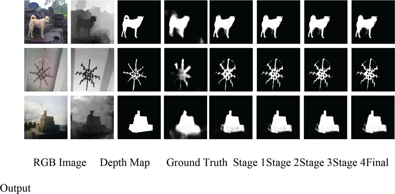
Figure 3:
Stage-wise optimization of extracted features has visualized the reconstruction of visual salient points in the low-depth images to predict the salient objects accurately.
d. Comparison and result analysis
We used four evaluation parameters; the proposed model is experimentally compared with 18 state-of-the-art SODs models. This comparison has made use of uniform parameters, testing, validation sets, and both quantitative and graphical evaluation. Recent, closely related, and extensively publicized literature served as the basis for the selection of state-of-the-art saliency in this comparison. The following state-of-the-art methods, HAIN [50], CASCNN [29], CoNet [51], DANet [19], cmMS [33], D3NET [20], CPFP [15], AFNet [26], CTMFR [27], PCANet [52], and DF [13], are closely related deep learning models. The summary of the findings from the analysis of the results is described below.
Quantitative Comparison: The computed results presented in Tables 1 and 2 demonstrate that the propos ed fea ture optimization strategy substantially enhanced all datasets utilizing the S-measures, E-measures, and F-measures, while also substantially reducing the MAE. The results were greatly enhanced by the feature optimization network, FAO, MFR, and SAM because contextual and modality-dependent features, high-level semantics, cross-complementary features, and optimized complementary features all work together to increase the saliency in crowded and complicated environments. The visual quantitative comparison using the PR-Curve and F-Measure parameters in LFSD and STERE data set is shown in Figure 5.
Table 1:
The quantitative comparison of the proposed model on six benchmark RGBD datasets with four recent evaluation parameters.
| Date-Set | Metric | OUR | Improving [53] | CATNet [54] | FCN [37] | AirSod [25] | MAD [55] | DCMF [56] | GCFNET [22] | HIFN [50] | CAS-GNN [29] | cmMS [33] | CoNet [51] | D3Net [20] | CPFP [15] | TANet [57] | PCFNET [52] | CTMF [27] | AFNet [26] | DF [13] |
|---|---|---|---|---|---|---|---|---|---|---|---|---|---|---|---|---|---|---|---|---|
| NJUD [6] | Fβ↑ | 0.945 | 0.940 | 0.929 | 0.918 | 0.918 | 0.903 | 0.888 | 0.915 | 0.915 | 0.893 | 0.914 | 0.872 | 0.900 | 0.877 | 0.874 | 0.872 | 0.845 | 0.775 | 0.804 |
| Sα↑ | 0.941 | 0.926 | 0.937 | 0.918 | 0.908 | 0.921 | 0.913 | 0.914 | 0.912 | 0.911 | 0.900 | 0.894 | 0.900 | 0.879 | 0.878 | 0.877 | 0.849 | 0.772 | 0.763 | |
| Eψ↑ | 0.969 | 0.959 | 0.933 | 0.953 | 0.944 | 0.930 | 0.925 | 0.947 | 0.944 | 0.922 | 0.914 | 0.912 | 0.950 | 0.926 | 0.925 | 0.924 | 0.913 | 0.853 | 0.864 | |
| MAE↓ | 0.024 | 0.026 | 0.025 | 0.039 | 0.034 | 0.037 | 0.043 | 0.038 | 0.038 | 0.036 | 0.044 | 0.047 | 0.041 | 0.053 | 0.060 | 0.059 | 0.085 | 0.100 | 0.141 | |
| NLPR [46] | Fβ↑ | 0.928 | 0.934 | 0.916 | 0.911 | 0.923 | 0.901 | 0.875 | 0.907 | 0.915 | 0.888 | 0.913 | 0.850 | 0.897 | 0.867 | 0.863 | 0.841 | 0.825 | 0.771 | 0.778 |
| Sα↑ | 0.949 | 0.932 | 0.939 | 0.924 | 0.908 | 0.933 | 0.922 | 0.919 | 0.924 | 0.919 | 0.899 | 0.907 | 0.912 | 0.888 | 0.886 | 0.874 | 0.860 | 0.799 | 0.802 | |
| Eψ↑ | 0.966 | 0.966 | 0.968 | 0.960 | 0.963 | 0.955 | 0.940 | 0.953 | 0.960 | 0.951 | 0.945 | 0.936 | 0.953 | 0.932 | 0.941 | 0.925 | 0.929 | 0.879 | 0.880 | |
| MAE↓ | 0.019 | 0.019 | 0.018 | 0.024 | 0.039 | 0.022 | 0.029 | 0.025 | 0.924 | 0.025 | 0.027 | 0.031 | 0.030 | 0.036 | 0.041 | 0.044 | 0.056 | 0.058 | 0.085 | |
| STEREO [47] | Fβ↑ | 0.945 | 0.933 | 0.902 | 0.906 | 0.900 | 0.892 | 0.872 | 0.900 | 0.906 | 0.876 | 0.908 | 0.885 | 0.891 | 0.871 | 0.861 | 0.860 | 0.831 | 0.823 | 0.757 |
| Sα↑ | 0.933 | 0.922 | 0.925 | 0.906 | 0.895 | 0.910 | 0.903 | 0.899 | 0.907 | 0.899 | 0.889 | 0.908 | 0.899 | 0.879 | 0.874 | 0.875 | 0.848 | 0.825 | 0.757 | |
| Eψ↑ | 0.967 | 0.953 | 0.935 | 0.947 | 0.939 | 0.939 | 0.930 | 0.940 | 0.944 | 0.929 | 0.922 | 0.922 | 0.938 | 0.925 | 0.923 | 0.925 | 0.912 | 0.887 | 0.847 | |
| MAE↓ | 0.031 | 0.026 | 0.030 | 0.032 | 0.043 | 0.037 | 0.043 | 0.040 | 0.040 | 0.039 | 0.042 | 0.041 | 0.046 | 0.051 | 0.060 | 0.064 | 0.086 | 0.075 | 0.141 | |
| SSD [48] | Fβ↑ | 0.889 | 0.861 | - | - | - | 0.850 | - | - | 0.870 | 0.840 | 0.865 | 0.806 | 0.834 | 0.766 | 0.810 | 0.807 | 0.729 | 0.687 | 0.735 |
| Sα↑ | 0.887 | 0.871 | - | - | - | 0.872 | - | - | 0.875 | 0.872 | 0.874 | 0.853 | 0.857 | 0.807 | 0.839 | 0.841 | 0.776 | 0.711 | 0.747 | |
| Eψ↑ | 0.940 | 0.917 | - | - | - | 0.907 | - | - | 0.917 | 0.915 | 0.911 | 0.896 | 0.910 | 0.852 | 0.897 | 0.894 | 0.865 | 0.807 | 0.828 | |
| MAE↓ | 0.042 | 0.045 | - | - | - | 0.045 | - | - | 0.045 | 0.047 | 0.052 | 0.059 | 0.058 | 0.082 | 0.063 | 0.062 | 0.099 | 0.118 | 0.142 | |
| LFSD [49] | Fβ↑ | 0.919 | 0.857 | 0.884 | 0.876 | - | 0.862 | 0.771 | 0.771 | 0.849 | 0.832 | 0.888 | 0.848 | 0.810 | 0.826 | 0.796 | 0.775 | 0.787 | 0.744 | 0.813 |
| Sα↑ | 0.909 | 0.821 | 0.894 | 0.875 | - | 0.867 | 0.879 | 0.846 | 0.845 | 0.846 | 0.846 | 0.862 | 0.825 | 0.828 | 0.801 | 0.786 | 0.788 | 0.738 | 0.783 | |
| Eψ↑ | 0.930 | 0.849 | 0.908 | 0.913 | - | 0.901 | 0.842 | 0.883 | 0.907 | 0.877 | 0.891 | 0.897 | 0.862 | 0.872 | 0.847 | 0.827 | 0.857 | 0.815 | 0.857 | |
| MAE↓ | 0.041 | 0.096 | 0.051 | 0.061 | - | 0.059 | 0.068 | 0.079 | 0.070 | 0.074 | 0.72 | 0.071 | 0.095 | 0.088 | 0.111 | 0.119 | 0.127 | 0.133 | 0.145 | |
| DUT-RGBD [5] | Fβ↑ | 0.960 | 0.859 | 0.951 | 0.931 | 0.920 | - | 0.928 | 0.923 | 0.913 | 0.912 | 0.932 | 0.908 | 0.867 | 0.795 | 0.790 | 0.771 | 0.823 | 0.659 | 0.744 |
| Sα↑ | 0.957 | 0.841 | 0.953 | 0.924 | 0.891 | - | 0.920 | 0.918 | 0.902 | 0.891 | 0.885 | 0.918 | 0.882 | 0.818 | 0.808 | 0.801 | 0.831 | 0.762 | 0.705 | |
| Eψ↑ | 0.977 | 0.879 | 0.971 | 0.956 | 0.946 | - | 0.950 | 0.951 | 0.929 | 0.932 | 0.940 | 0.941 | 0.889 | 0.859 | 0.861 | 0.856 | 0.899 | 0.796 | 0.823 | |
| MAE↓ | 0.020 | 0.071 | 0.020 | 0.032 | 0.048 | - | 0.043 | 0.040 | 0.041 | 0.043 | 0.036 | 0.034 | 0.061 | 0.076 | 0.093 | 0.100 | 0.097 | 0.122 | 0.145 |
Table 2:
Illustration of the contribution of optimization of each component of the proposed model.
| Setting | STEREO [47] | NJU2K [6] | LFSD [49] | |||||||||||||
|---|---|---|---|---|---|---|---|---|---|---|---|---|---|---|---|---|
| BASE MODEL | Low-depthissues | OUR | MFR | SAM | Fβ↑ | Sα↑ | Eψ↑ | MAE↓ | Fβ↑ | Sα↑ | Eψ↑ | MAE↓ | Fβ↑ | Sα↑ | Eψ↑ | MAE↓ |
| ✓ | 0.8038 | 0.8064 | 0.8572 | 0.0894 | 0.7559 | 0.7766 | 0.7703 | 0.1003 | 0.7095 | 0.7105 | 0.7090 | 0.1963 | ||||
| ✓ | ✓ | 0.8152 | 0.8334 | 0.8442 | 0.0840 | 0.7889 | 0.8690 | 0.8088 | 0.0900 | 0.7245 | 0.7505 | 0.7590 | 0.1083 | |||
| ✓ | ✓ | ✓ | 0.8481 | 0.8452 | 0.8555 | 0.0752 | 0.8245 | 0.8489 | 0.8505 | 0.0762 | 0.8335 | 0.8452 | 0.8580 | 0.0882 | ||
| ✓ | ✓ | ✓ | ✓ | 0.8582 | 0.8609 | 0.8781 | 0.0651 | 0.8772 | 0.8778 | 0.8780 | 0.0610 | 0.8676 | 0.8590 | 0.8775 | 0.0790 | |
| ✓ | ✓ | ✓ | ✓ | ✓ | 0.9456 | 0.9334 | 0.9674 | 0.0310 | 0.9456 | 0.9414 | 0.9698 | 0.0245 | 0.9197 | 0.9097 | 0.9370 | 0.0411 |
Visual Comparison: The computed saliency in cluttered and complicated backdrops is presented by the visual assessment in Figure 4. It shows the efficiency as compared to other models of stage-wise feature extraction with a composite backbone network and depth modality. The images shown in Figure 4 are cluttered backgrounds. Simultaneously, FAO eliminates the background while producing the salient objects with intact object structure. AF-Net, CTMFR, and PCAnet, in complex and cluttered backdrops, generate non-salient points due to their model lacking in extracting features in low-depth images. Although comparably better models CAS-CNN, D3NET, and CoNet performed poorly on the border region, generating some non-salient points as salient points. DCF, HAIN, DANet, and cmMS are shown much better to other models as shown in Figure 4.
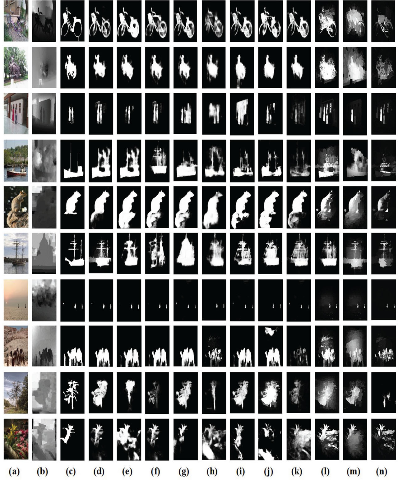
Figure 4:
The saliency maps is shown here for the visual demonstration (A) input RGB image, (B) depth image, (C) GT image, (D) OUR, (E) HAIN, (F) CAS−GNN, (G) cmMS, (H) CoNet, (I) D3NET, (J) CPSF, (K) TANet, (L) PCFNET, (M) CTMFR, and (N) AFNet of proposed model. GT, ground truth.
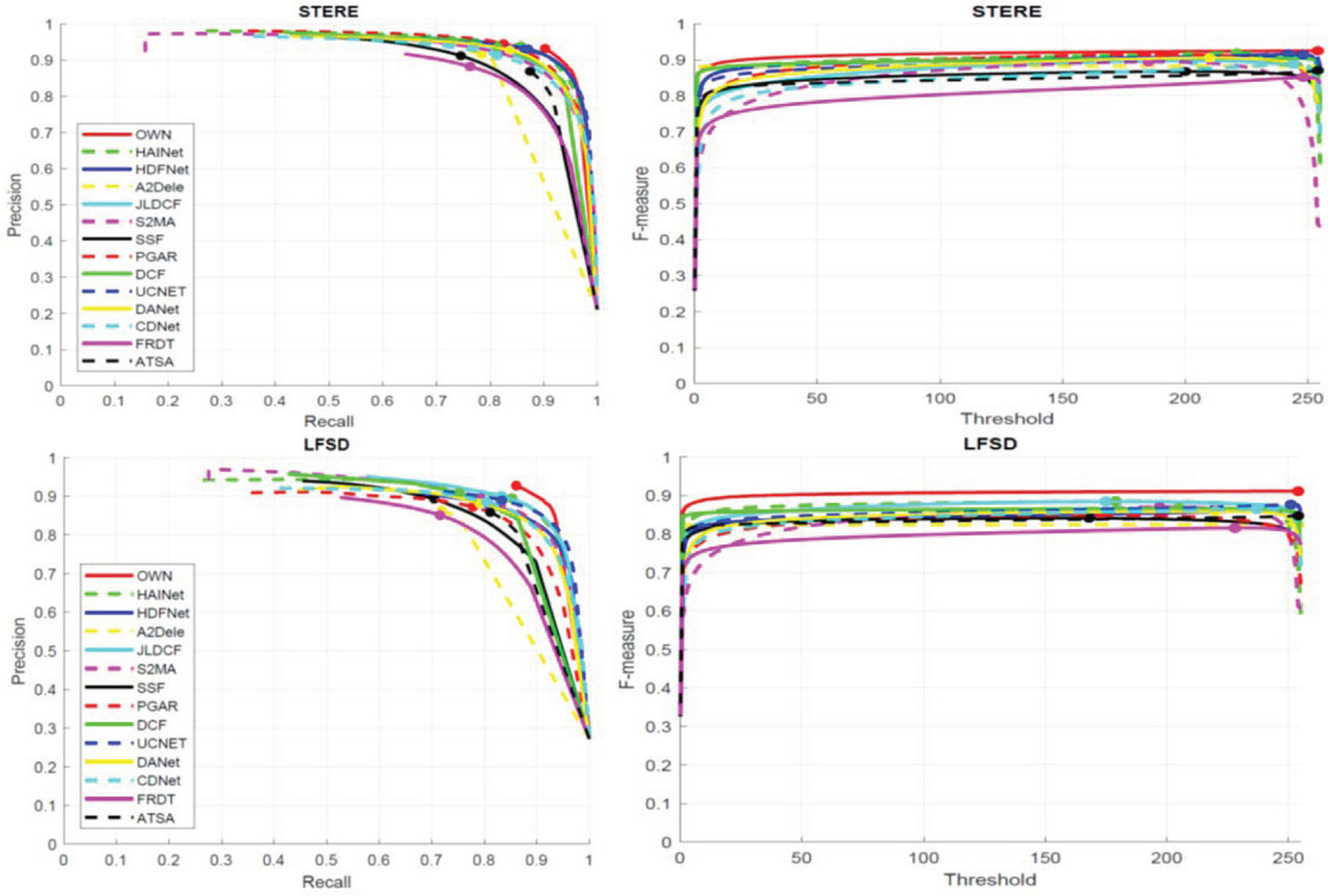
Figure 5:
Comparison of our proposed model with recent models with (A) PR-curve (B) F-measure (vertical axis (thresholds) and horizontal axis) datasets (1) STERE (2) LFSD dataset, respectively.
e. Ablation analysis
Ablation studies on six datasets using recent parameters and visual demonstration are used to investigate the contributions of each component in the proposed model. The effectiveness of the composite backbone network and the multi-horizon reconstruction mechanism is analyzed below.
1) Validation of Multi-horizon Reconstruction Mechanism: To validate saliency enhancement, a composite backbone network utilizing FAO based on the multi-horizon attention mechanism has to be proven effective. A simple model VGG-16 without stage-wise saliency fusion in a combined network. It cannot distinguish the salient and non-salient regions. The visual contribution of each step is shown in Figure 3. The effectiveness validation is measured through recent parameters, shown in Table 2. The successive contributions in saliency computations are shown in Table 2, which validates the effectiveness of each stream of FAO on complex RGBD-datasets. FAO is compared with a simple VGG-16 model without FAO, MFR, and SAM modules, which are shown in Table 2. The simple backbone produces independent saliency features which are not capable of predicting exact salient objects in complex images. At the same time, the FAO and MFR-based composite backbone network integrates both modalities-based salient features at each stage, which are shown in Figure 3. and in Table 2. While the SAM module minimizes the propagation of irrelevant features in the following stages, the MFR module improves the horizon of the feature domain, increasing the lost saliency feature.
V. Conclusion
A feature optimization with FAO, and MFR models, efficiently extracts the stage-wise optimal features. These stage-wise optimization features are efficiently fused using SAM modules to predict complex SOD. The multi-horizon attention mechanism utilized a spatial, channel-wise, cascaded, and combined attention mechanism-based optimization to enhance the saliency features. The MFR mechanism recovered the lost saliency in color and depth features in the four-fold dilated feature. It minimizes the propagation of irrelevant saliency while retaining all possible essential features to correct predictions and localization by improving low-depth issues and spatial coherence. Additionally, we designed an effective features exploration and reconstruction architecture by designing a task-specific search space for the multi-modal multiscale feature fusion. This model can be used in future in a variety of remote sensing and small target identification applications due to its broad future potential in identification in low-depth and complex background images.