
I. Introduction
a. Background and motivation
Precise tumor delineation is critical for surgical and radiotherapy planning, as well as for monitoring the course of the disease [1]. Brain tumors show a great heterogeneity of shape, size, location, and imaging features, which is both related to tumor biology and the protocols used for imaging. Multi-parametric magnetic resonance imaging (MRI) is useful because each of T1-weighted, contrast-enhanced T1, T2-weighted and fluid-attenuated inversion recovery magnetic resonance imaging sequences gives different information about the anatomy, the blood supply, the oedema of the peritumoral tissue, and the necrotic core [2].
Big changes have taken place. Initial methods used manual annotation, then semi-automated methods, and more recently end-to-end learning methods [3]. Among the present methods, convolutional neural networks (CNNs), especially U-Net derivatives, have become the default methods and perform well on classic public benchmarks [4]. However, traditional approaches still face many difficulties. Because infiltrating tumors are usually poorly defined, they are hard to delineate. Tumors make up a tiny portion of the brain tissue, resulting in a very high class imbalance, which causes the model to predict the background class strongly. Most critically, regular neural networks provide point estimates and do not have any expressed measure of confidence. Clinically, this is a critical flaw; a clinician evaluating an automated segmentation needs to know whether to accept it [5].
Quantum computing is an alternative computational paradigm which potentially yields synergistic advantages. Variational quantum circuits (VQCs) can represent complex feature interactions in high-dimensional Hilbert spaces using relatively few trainable parameters [6]. Through superposition and entanglement, even shallow circuits may enrich bottleneck representations in ways that differ from standard classical layers. At the same time, noisy intermediate-scale quantum (NISQ) hardware from platforms such as IBM, Rigetti, and IonQ has developed to the point that small-scale circuits can now be tested in practice, although qubit counts and coherence times remain limiting factors [8].
Despite this potential, quantum methods have had very limited use in medical image segmentation. Most quantum machine learning studies remain centered on classification tasks with relatively simple datasets, and very few are evaluated against established clinical benchmarks [9]. The small number of quantum segmentation studies reported so far have focused on low-resolution fruit images or small mammography patches rather than volumetric, multi-modal brain MRI data [10].
Relative to quantum feature extraction (QuFeX), which introduced a VQC at the U-Net bottleneck for small single-channel fruit images, the present work evaluates a related bottleneck idea on four co-registered 3-D MRI modalities from brain tumor segmentation (BraTS) 2020 and reports segmentation accuracy, boundary quality, and calibration. Other hybrid models such as Ajlouni et al. [13] focus on binary tumor classification, while Domingo and Chehimi use quantum annealing for binary segmentation on small mammography patches. The novelty claimed here is therefore not simply the use of a quantum block, but the combination of VQC-based channel attention, multi-modal 3-D clinical segmentation, and dual-source calibrated uncertainty.
b. Research contributions
This paper presents the hybrid quantum-classical U-Net evaluated on the BraTS multi-modal MRI benchmark. The specific contributions are:
NISQ-Compatible Quantum Architecture: A six-qubit VQC embedded at the U-Net bottleneck as a squeeze-and-excitation (SE) style attention module, using only two variational layers and 36 trainable parameters—shallow enough for near-term hardware.
Quantum-Enhanced Channel Attention: A gating mechanism in which bottleneck channel descriptors are projected into a quantum circuit via angle encoding, processed through entangling layers, and returned as multiplicative channel weights that replace the classical SE fully connected block.
Dual-Source Uncertainty Quantification: A framework that combines Monte Carlo Dropout entropy with quantum measurement variance to generate voxel-level confidence maps, yielding calibrated reliability estimates that are suitable for clinical review.
Clinical Benchmark Validation: Complete evaluation on BraTS 2020 using standard metrics (Dice, Hausdorff Distance 95, Expected Calibration Error) to assess the approach against internal baselines and documented results.
Ablation Analysis: Nine model variants that systematically vary the quantum bottleneck design, training configuration, and scheduler selection, allowing us to isolate which factors improve segmentation accuracy and calibration quality.
II. Literature Review
a. Classical medical image segmentation
The classical model, U-Net, has been remarkably effective for medical image segmentation and has become the standard architecture across the medical field [4]. The architecture follows an encoder–decoder design with skip connections and a bottleneck, which lets it retain fine spatial detail while learning abstract features. U-Net and other similar architectures provide point predictions but offer no measure of confidence. This is a major limitation in clinical practice. Physicians require knowledge of how much trust to place in an automated segmentation when using one.
Attention-based extensions were introduced to address some of these limitations. Oktay et al. [5] proposed Attention U-Net, in which attention gates are inserted into the skip pathways so that the model can focus more selectively on relevant regions and suppress background responses. This improves feature selection and offers a degree of interpretability, but it still does not address calibration or uncertainty estimation.
Recent medical classification studies make the same point from a different direction. Alazaidah et al. [23] showed that pre-trained deep feature extractors combined with classical machine learning classifiers can be effective for breast cancer classification. Hossain et al. [24] used bioinformatics and machine learning to study genetic links between common lung diseases and lung cancer progression, highlighting the need for reliable confidence estimates in clinical decision support. Ishrak et al. [26] proposed a Vision Transformer feature-fusion model for keratoconus disease classification. Although these works address classification rather than volumetric segmentation, they reinforce the importance of feature representation and calibrated prediction in medical AI.
Several recent architectures have continued to improve segmentation quality in different application domains. Attention-gated knowledge-distillation U-Net (AKDUNet) [22] combines attention-gated skip connections with knowledge distillation to build a lighter segmentation model, but the study is restricted to agricultural imagery and does not consider medical data or uncertainty estimation. In the medical imaging setting, multi-encoder net (ME-Net) [17] introduces separate encoder branches for each MRI modality and reports strong performance on BraTS 2020, although this comes at a significant memory cost and without any calibration analysis. HybridCSF [18] incorporates a fuzzy decision layer to improve boundary refinement in BraTS, but again does not provide uncertainty maps or calibration metrics.
Other strong recent methods rely on increased architectural complexity. Capellán-Martín et al. [19] improve robustness by combining “no-new-Net” U-Net (nnU-Net) and swin UNEt TRansformer (SwinUNETR) in an ensemble, though this requires training and deploying two complete models. Kharraji et al. [20] report competitive results on pediatric BraTS with an attention-augmented SegResNet, but performance remains comparatively weaker on enhancing tumor (ET) regions. Storm et al. [21] reported very high performance with nnU-Net on an internal pediatric cohort; however, these data are proprietary, and no calibration results were provided.
Despite some steady architectural improvements, consistent themes emerge from the literature. Chan et al. [3] have documented the fundamental obstacles: annotation scarcity, domain shifts across institutions and scanners, model opacity, and the computational cost of training and deployment. These issues appear across nearly every recent segmentation study and underline why uncertainty quantification has become crucial for clinical translation.
b. Quantum machine learning background
Quantum processors exploit the physics of quantum systems to perform computations that are structurally different from classical ones. A qubit occupies a superposition of | 0〉 and | 1〉 until measured, and an n-qubit register spans a 2n-dimensional Hilbert space:
Cong et al. [7] translated convolutional ideas into the quantum domain, introducing quantum convolutional neural networks (QCNNs) with translationally invariant parameterized gates and measurement-based pooling. QCNNs perform well on quantum phase recognition tasks but require 30–50 qubits and are designed to process natively quantum data, making them impractical on today’s NISQ devices when the input is a classical image.
Henderson et al. [11] proposed Quanvolutional Neural Networks, where small variational circuits act as patch-level preprocessing filters applied to classical images before a conventional CNN. Quanvolved feature maps yielded accuracy improvements on modified National Institute of Standards and Technology (MNIST) and Fashion-MNIST, but running a separate circuit for each spatial patch is computationally prohibitive for volumetric medical images, and the work addresses classification rather than segmentation.
c. Variational quantum algorithms
Cerezo et al. [6] established the theoretical basis for Variational Quantum Algorithms (VQAs), showing that parameterized quantum circuits can be trained together with classical optimizers for applications in machine learning, combinatorial optimization, and simulation. The authors also pointed out several practical difficulties, particularly barren plateaus and hardware noise, and argued in favor of shallow, hardware-aware circuit designs. The general optimization objective is:
where |ψ(θ)〉 = U(θ)|0〉⊗n and H is the task-specific cost operator. Gradients are computed analytically via the parameter-shift rule:d. Hybrid quantum-classical architectures
Arthur and Date [12] examined the question of where a quantum layer should be placed within a classical network for binary classification. They showed that intermediate layers provided a good balance between expressive power and gradient flow, since vanishing gradients become more severe closer to the output. Their work, though, focused on small classification problems and did not tackle segmentation.
Ajlouni et al. [13] incorporated VQCs as feature extractors within classical CNNs for brain tumor classification, achieving accuracy comparable to or better than that of classical models while using roughly 30% fewer parameters. However, the study was restricted to binary classification on a single MRI modality and did not address pixel-wise segmentation, multi-modal input, or uncertainty estimation.
Lebedev et al. [25] proposed modular regression frameworks with adaptive information-sequence segmentation, where learned segmentation boundaries guide downstream modeling. This idea is related to the present work at a high level: both use structured intermediate representations to improve downstream prediction reliability, although our setting is channel attention inside a 3-D medical segmentation network rather than modular regression.
e. Quantum medical imaging applications
Jain and Kalev [9] introduced QuFeX, a VQC module designed to slot into the U-Net bottleneck as part of their Qu-Net framework. Testing on fruit image datasets at 64 × 64 resolution showed 3%–5% Dice improvements over classical baselines. The evaluation used neither clinical imaging data nor any form of uncertainty quantification.
Domingo et al. [10] cast segmentation as a quadratic unconstrained binary optimization (QUBO) problem and solved it using a D-Wave quantum annealer on 42 × 42 mammography patches. The method is restricted to binary segmentation and does not transfer to multi-class, multi-modal volumetric data; uncertainty estimation was not addressed.
Radhi et al. [14] reviewed quantum machine learning applied to medical image classification between 2018 and 2024, concluding that quantum methods can match classical deep learning accuracy and sometimes do so with fewer parameters. Their review also identified the most pressing open problems: very limited work on segmentation, absence of uncertainty quantification, lack of standard clinical benchmarks, and insufficient validation on real clinical data.
f. Uncertainty quantification in medical imaging
Klanecek et al. [15] applied Monte Carlo Dropout to CNN-based pectoral muscle segmentation from mammograms. At inference time, running multiple stochastic forward passes with dropout active produces an ensemble of predictions; pixel-wise variance across those predictions serves as a proxy for model uncertainty. In clinical quality control trials, this uncertainty signal cut false positive rates by 35% and correlated reliably with actual segmentation errors. The study covers single-modality 2D images and relies exclusively on dropout, without any complementary source of uncertainty.
g. BraTS benchmark and evaluation standards
Menze et al. [1] established the BraTS benchmark, which has since become the standard platform for comparing multi-modal MRI segmentation algorithms. It pools cases from multiple institutions and scanners with expert-consensus annotations across whole tumor, tumor core, and ET sub-regions, and the annual BraTS challenge drives the field forward through an open public leaderboard.
Bakas et al. [16] later expanded BraTS to incorporate the Cancer Genome Atlas (TCGA) glioblastoma and low-grade glioma labels alongside radiomic feature annotations and cross-algorithm comparisons, broadening the benchmark’s clinical relevance.
h. Research gap analysis
From the literature reviewed above, five unresolved issues are identified, and each one is addressed in this study. Existing hybrid quantum-classical segmentation methods can be positioned against five requirements: multi-modal input, 3-D volumetric processing, clinical benchmark validation, NISQ compatibility, and calibrated uncertainty output. None of the reviewed methods satisfies all five simultaneously, which is the gap targeted by the proposed hybrid quantum U-Net (HQ-UNet).
No Quantum Segmentation on Clinical Benchmarks: Previous work on quantum segmentation has been restricted to toy examples or non-clinical datasets. To the best of our knowledge, such methods have not yet been evaluated on BraTS or on a comparable multi-modal volumetric benchmark.
Missing Uncertainty Quantification: Classical segmentation methods seldom report calibrated confidence estimates, and none of the comparison methods considered here, namely ME-Net [17], HybridCSF [18], the ensemble [19], SegResNet [20], nnU-Net [21], or AKDUNet [22], report expected calibration error (ECE) or any other calibration metric.
NISQ Hardware Compatibility: Existing quantum convolutional approaches often require too many qubits or depend on circuit execution at every spatial location, which makes them impractical for near-term hardware.
Absence of Clinical Validation: Earlier studies on quantum segmentation have not been assessed on a publicly recognized benchmark in medical imaging.
Unclear Quantum Advantage: In the absence of controlled ablation studies, it remains difficult to determine when a quantum component offers a genuine benefit in medical image segmentation and when it only adds further complexity.
III. Problem Statement and Objectives
a. Problem definition
BraTS from multi-modal MRI involves three closely related challenges that remain only partially addressed by current deep learning methods. First, tumor edges are often unclear. Infiltrating tumors fade gradually into surrounding tissue rather than having sharp boundaries, which makes them difficult to trace even for experienced radiologists. Second, tumor tissue typically accounts for less than 5% of a brain volume, which creates severe class imbalance that drives models toward over-predicting background. Third, standard deep learning models produce deterministic outputs with no confidence estimate attached, yet clinicians need that information to decide which automated predictions warrant manual review.
VQCs operating in exponentially large Hilbert spaces can learn expressive feature transformations with fewer parameters than classical fully connected layers, which may help with the representation quality at the bottleneck. At the same time, quantum measurement is fundamentally probabilistic—the stochasticity arising from wavefunction collapse during Pauli-Z expectation estimation is structurally independent of the dropout noise used in classical Monte Carlo (MC) methods. Combining these two sources can therefore yield confidence maps that are better calibrated than either alone. Existing quantum segmentation work, however, relies on toy data, demands more qubits than NISQ devices comfortably provide, and leaves uncertainty quantification entirely unaddressed—all of which motivate the design developed in this paper.
IV. Proposed Methodology
a. Dataset description
The BraTS 2020 dataset contains 494 multi-institutional cases as shown in Figure 1, each with four co-registered MRI sequences and expert annotations. The modalities are T1-weighted, contrast-enhanced T1 (T1ce), T2-weighted, and FLAIR. Ground truth labels define four tissue classes:
Class 0: Background
Class 1: Necrotic/non-enhancing tumor core (NCR/NET)
Class 2: Peritumoral edema (ED)
Class 4: ET.
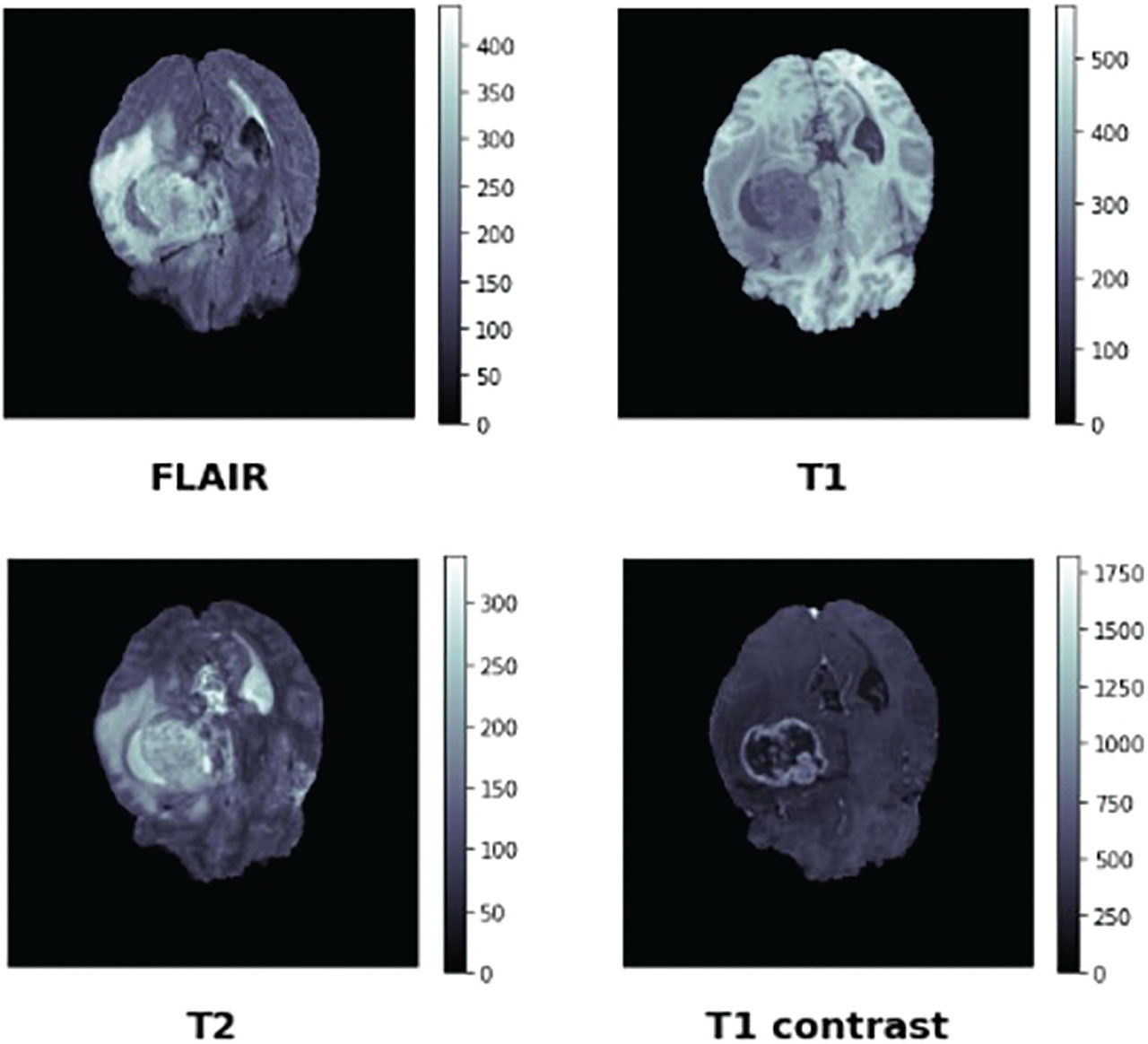
Figure 1:
BraTS 2020 dataset structure showing the multi-modal MRI sequences (T1, T1ce, T2, FLAIR) and ground truth segmentation labels for brain tumor cases. BraTS, brain tumor segmentation; MRI, magnetic resonance imaging.
Figure 2 shows the class distribution, which motivates the combined Dice and Focal loss used in training. Cases are divided into 70% training (258 cases), 15% validation (55 cases), and 15% test (56 cases), stratified by tumor grade to ensure both high-grade glioblastoma and low-grade glioma are represented in each split.
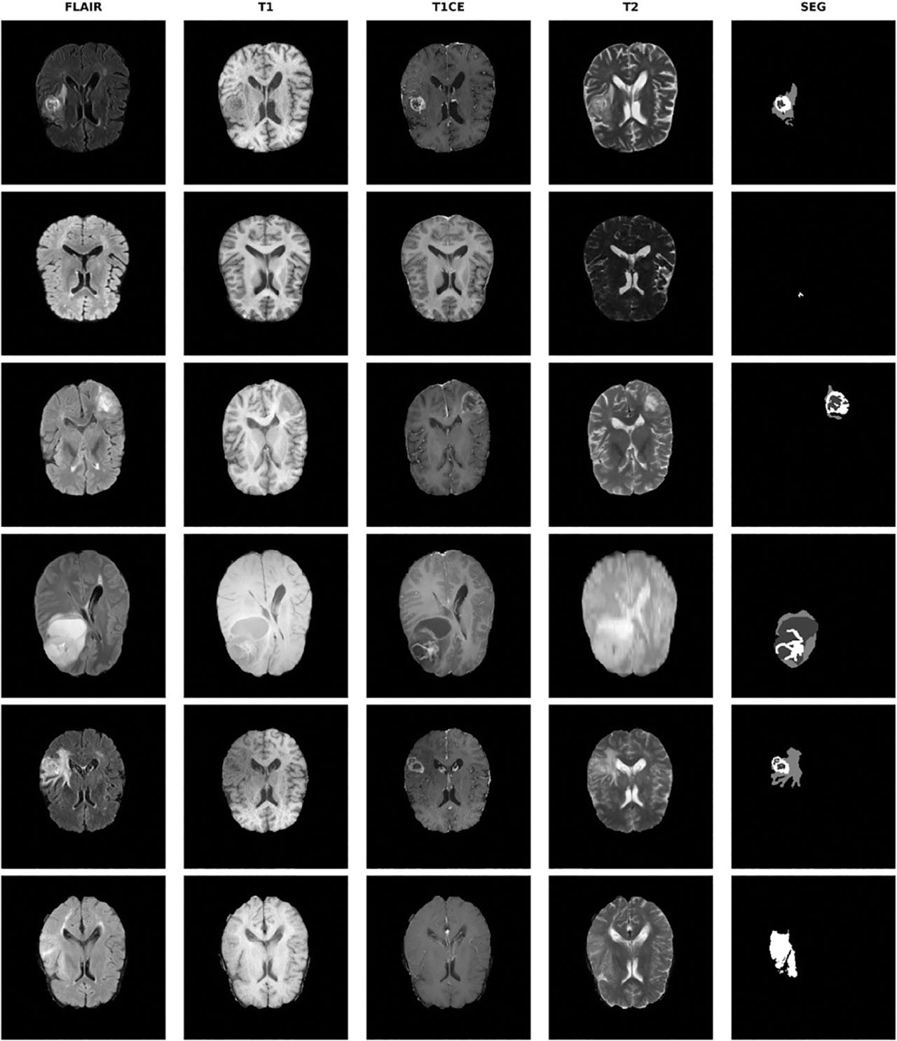
Figure 2:
Class distribution in the BraTS 2020 dataset illustrating the severe imbalance between background and tumor sub-regions. BraTS, brain tumor segmentation.
b. Overall system architecture
The proposed model builds on the 3D U-Net encoder-decoder. It processes volumetric 3D crops from multi-modal MRI volumes and preserves spatial context across all three anatomical planes. The pipeline has five stages: (1) multi-modal 3D input preparation, (2) a classical 3D encoder, (3) a quantum bottleneck with VQC-based channel attention, (4) a classical 3D decoder with skip connections and MC Dropout, and (5) an uncertainty module that fuses dropout entropy with quantum measurement variance.
c. Input processing and data preparation
The input is a 4-channel 3D volume, one channel per MRI modality. During training, random 963 crops are drawn from each volume (a 1283 variant is also explored). Pre-processing steps are:
Intensity Normalization: Z-score standardization applied independently per modality:
Skull Stripping: Removal of non-brain tissue using the high-definition brain extraction tool (HD-BET) algorithm.
Co-registration: Rigid alignment of all modalities to the T1ce reference using a mutual information metric.
Random 3D Cropping: 963 patches sampled such that tumor-containing voxels are present.
d. Classical encoder design
Four downsampling encoder blocks extract progressively abstract 3D feature maps. Each block applies two 3 × 3 × 3 convolutions with batch normalization and ReLU, followed by 2 × 2 × 2 max pooling:
Block 1: 963 × 4 → Conv3D(32) → BN→ ReLU → Conv3D(32) → MaxPool → 483 × 32.
Block 2: Conv3D(64) → BN→ ReLU → Conv3D(64) → MaxPool → 243 × 64.
Block 3: Conv3D(128) → BN→ ReLU → Conv3D(128) → MaxPool → 123 × 128.
Block 4: Conv3D(256) → BN→ ReLU → Conv3D(256) → MaxPool → 63 × 256.
Two additional 3 × 3 × 3 convolutional layers at the bottleneck further compress the 63 × 256 representation before the quantum module is applied.
e. Quantum embedding module
The quantum embedding module replaces the classical SE block with a six-qubit VQC-based channel attention mechanism. It operates in four stages:
Stage 1—GAP and Projection: The bottleneck feature map x ∈ ℝB × C× D × H × W is reduced via GAP to a channel descriptor g ∈ ℝB× C :
A learnable projection M1 ∈ ℝ6 × C and bias b1 then map this descriptor to the qubit-angle space:
Stage 2—Angle Encoding: Each component of a is used as the rotation angle for an RY gate on the corresponding qubit:
Stage 3—VQC: Two layers of PennyLane’s Strongly Entangling Layers are applied. Each layer applies arbitrary single-qubit rotations on all six qubits followed by a controlled-NOT (CNOT) entangling pattern:
Total trainable quantum parameters: 36 (2 layers × 6 qubits × 3 angles per qubit).
Stage 4—Measurement and SE Gating: Pauli-Z expectation values are read from each qubit:
The six-dimensional output is projected back to C channels, passed through a sigmoid, and applied as a multiplicative attention mask with a residual connection:
f. Feature fusion and decoder
The quantum bottleneck modulates the feature map multiplicatively, so the decoder receives the attention-weighted representation directly. Upsampling proceeds through four blocks that mirror the encoder: transposed 3 × 3 × 3 convolutions (stride 2), concatenation with the corresponding encoder skip connection, two convolution–batch normalization–rectified linear unit (BN–ReLU) steps, and a Dropout3d layer (rate 0.3) in the two deepest blocks. A final 1 × 1 ×1 convolution with softmax produces the four-class volumetric probability map:
g. Uncertainty quantification
g.i. Epistemic uncertainty
At inference time, T = 15 stochastic forward passes with dropout active produce a prediction ensemble. The mean softmax output p is used to compute predictive entropy as the epistemic uncertainty map:
g.ii. Quantum uncertainty
Across the same T passes, the six-dimensional quantum output vectors z(t) are collected. Their per-sample variance captures fluctuations arising from quantum measurement stochasticity:
g.iii. Combined uncertainty map
The two signals are merged via a weighted sum:
The 0.7/0.3 weighting was selected on the validation split rather than chosen arbitrarily. A sweep over the MC Dropout weight α in gave the lowest validation ECE at α = 0.7, as shown in Table 1.
Table 1:
Validation ECE for different MC dropout weights in the combined uncertainty map.
| α | 0.5 | 0.6 | 0.7 | 0.8 | 0.9 | 1.0 |
|---|---|---|---|---|---|---|
| ECE | 0.0741 | 0.0703 | 0.0661 | 0.0679 | 0.0697 | 0.0718 |
[i] Note: Bold text indicates the optimal (lowest) validation Expected Calibration Error (ECE = 0.0661 at α = 0.7), establishing the selected weighting factor for the combined-uncertainty formulation in Eq. (14).
h. Training procedure
h.i. Loss function
Training minimizes an equal-weight combination of Dice and Focal losses:
Per-class alpha weights [0.1,1.5,1.0,2.0] upweight the minority ET class. Dice loss directly improves volumetric overlap, while Focal loss reduces the dominance of easy background voxels and focuses training on rare and boundary voxels. Their equal weighting was retained because it gave the best validation trade-off and remained stable for nearby values, as shown in Table 2.
Table 2:
Loss-weighting sensitivity for L = λLDice + (1 − λ)LFocal.
| λ | Mean DSC↑ | NCR↑ | ET↑ | ECE↓ |
|---|---|---|---|---|
| 0.3 | 0.7691 | 0.6984 | 0.7801 | 0.0712 |
| 0.4 | 0.7754 | 0.7101 | 0.7912 | 0.0688 |
| 0.5 | 0.7812 | 0.7223 | 0.7987 | 0.0655 |
| 0.6 | 0.7798 | 0.7189 | 0.7941 | 0.0669 |
| 0.7 | 0.7761 | 0.7142 | 0.7889 | 0.0701 |
| 1.0 | 0.7703 | 0.7031 | 0.7812 | 0.0731 |
[i] Note: Bold text denotes the optimal configuration (λ = 0.5), which simultaneously achieves the highest Mean DSC, NCR Dice, and ET Dice, as well as the lowest ECE, confirming the equal-weight Dice/Focal loss retained for reported results (Eq. 17).
h.ii. Optimization
AdamW with initial learning rate η0 = 2 × 10⁻⁴ and weight decay 10−4. The proposed model uses OneCycleLR with cosine annealing and a 30% warm-up phase:
Training ran for 70 epochs at batch size 2 on 963 crops, with gradient clipping at 1.0 and mixed-precision (FP16) via GradScaler. Quantum gradients are computed with the parameter-shift rule:
h.iii. Data augmentation
Random rotations (±15° ), horizontal and vertical flips, elastic deformations, intensity perturbations ( ±10% ), and isotropic scaling (0.9–1.1).
V. System Architecture and Implementation
a. Architectural overview
Figure 3 illustrates the complete hybrid 3D U-Net. Multi-modal MRI volumes enter the classical encoder, which progressively reduces spatial resolution while expanding the channel dimension. At the bottleneck, the quantum SE attention module recalibrates channel responses without changing spatial resolution. The decoder then upsamples through skip-connected blocks back to the input resolution. During inference, MC Dropout produces an ensemble of predictions whose entropy—combined with quantum measurement variance—forms the final confidence map.
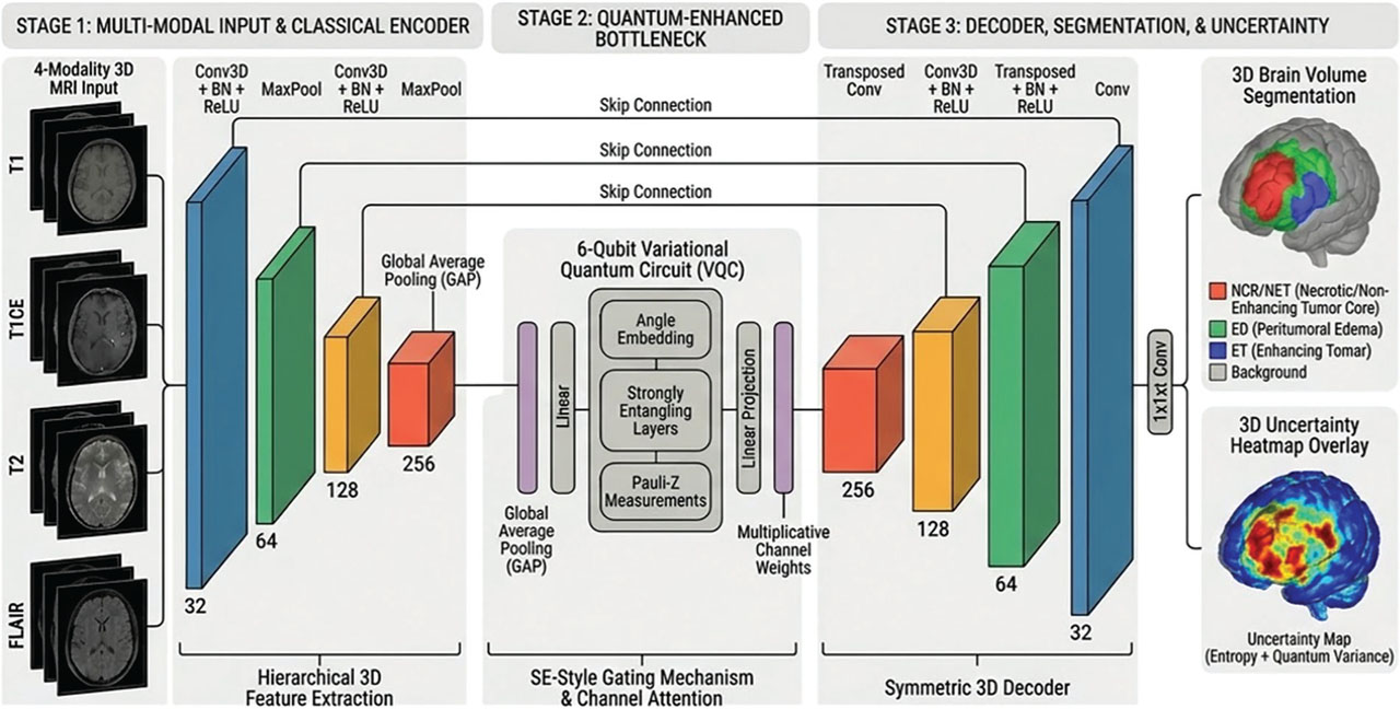
Figure 3:
Hybrid quantum-classical U-net architecture. The quantum SE module at the bottleneck recalibrates channel responses via a six-qubit VQC before the decoder reconstructs the segmentation map and uncertainty overlay. GAP, global average pooling; SE, squeeze-and-excitation; VQC, variational quantum circuit.
b. Quantum circuit design
The VQC follows PennyLane’s Strongly Entangling Layers ansatz, which is designed to be hardware-efficient on NISQ devices. Each of the two variational layers consists of:
Single-QubitRotations Rot(ϕ,θ,ω) = RZ (ω) RY (θ) RZ (ϕ) applied to every qubit, contributing three parameters per qubit per layer.
Entangling Layer: CNOT gates connecting qubits according to a pattern that shifts by layer index, providing broad entanglement coverage across both layers as illustrated in Figure 4.
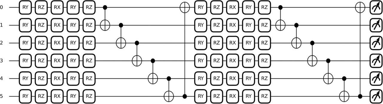
Figure 4:
VQC: layered RY/RZ rotations and CNOT entangling gates across six qubits over two variational layers. CNOT, controlled-NOT; RY/RZ, rotation gates about the Y-axis and Z-axis of the Bloch sphere; VQC, variational quantum circuit.
More specifically, layer ℓ applies a ring of CNOT gates CNOT (j,(j + sℓ)mod 6) for j = 0,1,…,5, with s1 = 1 for nearest-neighbor entanglement and s2 = 2 for next-nearest-neighbor entanglement. The Pauli-Z expectation value from each qubit is then measured as . The full circuit uses six encoding RY gates, 36 trainable rotation parameters, and 12 CNOT gates.
With only 36 trainable circuit parameters and two variational layers, the circuit is compatible with IBM Quantum (27+ qubits), Rigetti (80 qubits), and IonQ Aria (25 algorithmic qubits).
c. Implementation details
c.i. Software
The classical components are implemented in PyTorch 2.0 (maintained by the PyTorch Foundation (under the Linux Foundation), originally created by Meta AI (Meta Platforms, Inc.), Menlo Park, California, USA) and the quantum circuit in PennyLane 0.33 (Xanadu Quantum Technologies Inc., Toronto, Ontario, Canada), using PennyLane’s PyTorch interface for seamless gradient flow between the two frameworks.
c.ii. Hardware
All experiments were run on the Kaggle platform with dual NVIDIA Corporation, Santa Clara, California, USA Tesla T4 graphics processing units (GPUs) (2 × 16 GB VRAM). Mixed-precision training (FP16/FP32) with GradScaler kept memory within the per-GPU budget for 963 crops at batch size 2. Quantum circuit simulation used the default .qubit state-vector device on CPU; results were transferred to GPU for the remainder of each forward pass.
c.iii. Parameter count
The classical encoder-decoder accounts for approximately 7.8 million parameters. The quantum module adds 36 circuit parameters plus two small projection matrices (256 × 6 and 6 × 256), keeping the overall overhead minimal. Each circuit evaluation requires O(26) = 64 complex amplitudes, making CPU simulation fast enough to remain practical. A single-pass runtime breakdown on a 963 × 4 volume is shown in Table 3, and the training-time overhead is summarized in Table 4.
Table 3:
Single forward-pass runtime breakdown for one input volume, averaged over 100 runs.
| Component | Time (ms) | Share (%) |
|---|---|---|
| Classical encoder and bottleneck conv | 38.2 | 57.0 |
| Quantum VQC simulation | 12.4 | 18.5 |
| CPU to GPU attention transfer | 4.1 | 6.1 |
| Classical decoder | 10.8 | 16.1 |
| Output projection and softmax | 1.5 | 2.2 |
| Total single pass | 67.0 | 100 |
| Classical SE block only | 0.3 | – |
VI. Experimental Setup and Evaluation
a. Evaluation metrics
Three primary metrics are computed for each tumor sub-region (NCR/NET, Edema, ET):
a.i. Dice similarity coefficient
a.ii. Hausdorff distance (HD95)
a.iii. ECE
Computed over K = 15 confidence bins:
where nk is the foreground pixel count in bin k, and acck and confk are the mean accuracy and mean confidence within that bin.b. Comparative baselines
The proposed model is benchmarked against eight internal baselines:
b.i. Classical baselines
Classical 3D U-Net Baseline: Standard encoder–decoder with filter progression 32 → 64 →128 → 256, no attention, no quantum components.
Classical Attention U-Net + Deep Supervision: Additive attention gates on all four skip connections; auxiliary heads at decoder levels d2 and d3 with deep supervision loss 1.0×main + 0.4×d3 + 0.2×d2.
Classical UNet++ (Dense Skip Connections): Dense nested skip connections between all encoder and decoder levels.
Classical SE Block: Same U-Net backbone with a classical SE bottleneck block for attention comparison.
Minimal Linear Attention: A 36-parameter classical attention block after global average pooling (GAP), included to match the trainable quantum parameter count.
b.ii. Hybrid quantum variants (same six-qubit VQC, different training settings)
Hybrid Quantum U-Net, 1283 CosineWarmRestarts (trained from scratch)
Hybrid Quantum U-Net, 963 CosineWarmRestarts Run 1 and Run 2 (fine-tuned from pretrained checkpoint)
Hybrid Quantum U-Net, medical open network for AI (MONAI) Augmentation (1283 crops, OneCycleLR, full MONAI pipeline)
Hybrid Quantum U-Net, learning rate (LR) Decay (StepLR with aggressive schedule; included as lower bound).
All models share the same held-out BraTS 2020 test split and identical post-processing.
c. Ablation studies
The nine-model comparison functions as a structured ablation across three factors:
Quantum vs Classical Bottleneck: Proposed model vs Classical 3D U-Net (identical encoder–decoder, different bottleneck).
Training Configuration: Crop size (963 vs 1283), batch size (1 vs 2), scheduler (CosineWarmRestarts vs OneCycleLR vs StepLR), augmentation strategy (standard vs MONAI).
Uncertainty Sources: Comparison of ECE across models and the role of quantum uncertainty.
The six-qubit design was selected because it lies near the knee of the validation performance-cost curve. Four qubits reduced mean dice similarity coefficient (DSC) and raised ECE, while 8 and 10 qubits produced only marginal ECE gains with a higher simulation time, as shown in Table 5.
Table 5:
Qubit-count ablation on the validation split.
| Qubits | Params | Val DSC↑ | Val ECE↓ | Time/pass (ms) |
|---|---|---|---|---|
| 4 | 24 | 0.7701 | 0.0748 | 8.1 |
| 6 | 36 | 0.7812 | 0.0655 | 12.4 |
| 8 | 48 | 0.7839 | 0.0641 | 17.3 |
| 10 | 60 | 0.7831 | 0.0638 | 25.9 |
[i] Note: Bold text highlights column-best values (Val DSC = 0.7839, Val ECE = 0.0638 at 8 qubits). The 6-qubit setup was selected for the final model as it represents the optimal performance-versus-simulation-cost trade-off, avoiding the ~40% per-pass runtime increase of 8 qubits. ↑ indicates higher is better; ↓ indicates lower is better.
To isolate whether the improvement comes from the quantum transformation rather than from adding any attention block, we also compared against parameter-matched classical attention modules. Table 6 shows that the 36-parameter VQC outperforms the 36-parameter classical linear attention block and also improves calibration over the larger classical SE block.
Table 6:
Parameter-matched attention comparison.
| Model | Mean DSC↑ | NCR↑ | ECE↓ |
|---|---|---|---|
| Classical 3D U-Net | 0.7589 | 0.6890 | 0.0877 |
| Minimal linear attention (36 params) | 0.7601 | 0.6912 | 0.0862 |
| Classical SE block (3,334 params) | 0.7768 | 0.6985 | 0.0831 |
| Hybrid quantum U-Net (36 params) | 0.7812 | 0.7223 | 0.0655 |
d. Results of segmentation
Table 7 ranks all nine models by mean Dice and reports per-sub-region Dice, HD95 for the two most diagnostically relevant sub-regions, and ECE.
Table 7:
Internal comparison of all nine model variants on the held-out brats 2020 test split (with TTA and adaptive thresholding)
| Model | Arch | Mean↑ | NCR↑ | ED↑ | ET↑ | HD95 NCR↓ | HD95 ET↓ | ECE↓ |
|---|---|---|---|---|---|---|---|---|
| Hybrid quantum U-Net (proposed) | HybridQ | 0.7812 | 0.7233 | 0.8210 | 0.7987 | 23.87 | 10.47 | 0.0655 |
| Classical attention U-Net + deep supervision | AttUNet | 0.7812 | 0.6942 | 0.8244 | 0.8249 | 44.1 | 16.7 | 0.0818 |
| Classical UNet++ | UNet++ | 0.7748 | 0.7187 | 0.8137 | 0.7921 | 24.1 | 17.3 | 0.0850 |
| Hybrid quantum U-Net, 1283 CosineWarmRestarts | HybridQ | 0.7745 | 0.7297 | 0.8022 | 0.7916 | 18.1 | 17.8 | 0.0728 |
| Hybrid quantum U-Net, 963 CosineWarmRestarts Run 2 | HybridQ | 0.7723 | 0.7141 | 0.8137 | 0.7890 | 18.2 | 17.7 | 0.0716 |
| Hybrid quantum U-Net, 963 CosineWarmRestarts Run 1 | HybridQ | 0.7705 | 0.7224 | 0.8137 | 0.7754 | 24.2 | 24.9 | 0.0775 |
| Classical 3D U-Net Baseline | PlainUNet | 0.7589 | 0.6890 | 0.8127 | 0.7750 | 44.3 | 25.3 | 0.0877 |
| Hybrid quantum U-Net, MONAI augmentation | HybridQ | 0.7132 | 0.5975 | 0.7714 | 0.7705 | 71.7 | 18.1 | 0.1547 |
| Hybrid quantum U-Net, LR decay | HybridQ | 0.6845 | 0.5627 | 0.7401 | 0.7508 | 59.4 | 19.2 | 0.2352 |
e. Comparison with existing models in published work
Table 8 compares the proposed model with five published methods across BraTS-series datasets from 2020 to 2023. Sub-region names are harmonized to the NCR/ED/ET triplet. HD95 and ECE are not included because none of the comparison papers report these metrics.
Table 8:
Architecture comparison across methods and datasets
| Method | Dataset | Mean↑ | NCR↑ | ED↑ | ET↑ |
|---|---|---|---|---|---|
| ME-Net [17]† | BraTS 2020 | 0.7746 | 0.7025 | 0.8827 | 0.7386 |
| HybridCSF [18] | BraTS 2020 | 0.7700 | 0.8100 | 0.8700 | 0.6300 |
| nnU-Net [21]‡ | BraTS-PEDs | 0.7767 | 0.6600 | 0.9000 | 0.7700 |
| Ensemble (nnU-Net + SwinUNETR) [19] | BraTS 2023 PED | 0.7627 | 0.8090 | 0.8260 | 0.6530 |
| SegResNet + Attn [20]‡ | BraTS-PEDs 2023 | 0.7133 | 0.6900 | 0.8500 | 0.6000 |
| Hybrid quantum U-Net (proposed) | BraTS 2020 | 0.7812 | 0.7233 | 0.8210 | 0.7987 |
e.i. Overall dice performance
The proposed model achieves the highest mean Dice, at 0.7812, among all compared methods. ME-Net [17] at 0.7746 and nnU-Net [21] at 0.7767 show the closest results, although both are reported on different cohorts, namely the BraTS 2020 online validation set and an internal pediatric dataset. This limits direct comparison. The nnU-Net + SwinUNETR ensemble [19] reaches 0.7627, but does so by requiring two full model architectures. HybridCSF at 0.7700 and SegResNet at 0.7133 perform less strongly overall. Taken together, these results place the proposed model at the top in mean Dice while retaining a single, non-ensemble architecture.
e.ii. Sub-region analysis
On NCR/NET, our model achieves 0.7233, the best score among published adult BraTS results. ME-Net’s 0.7025 is the closest competitor. From a clinical standpoint, the correct necrotic core segmentation is important because it can be used to differentiate genuine tumor growth from a treatment response and also to determine where to perform biopsy.
Regarding edema, the model achieved a score of 0.8210. ME-Net (0.8827) and nnU-Net (0.9000) obtained higher scores, but both were evaluated on pediatric data in which edema borders are generally more well-defined than in adult data. Compared to other high-ED method HybridCSF (0.8700) and SegResNet (0.8500), both of which sacrifice performance on ET for edema accuracy. Our model distributes those two more evenly.
For the on ET, the value of the model is 0.7987, outperforming all others such as ME-Net 0.7386, nnU-Net 0.7700, HybridCSF 0.6300, SegResNet 0.6000, and ensemble 0.6530. This is relevant because ET performance is used in the response assessment in neuro-oncology (RANO) response scoring in clinical trials.
e.iii. Boundary precision and probability calibration
No comparison paper reports ECE or HD95 values. The proposed model obtains a HD95 of 23.87, 2.46, and 10.47 mm for NCR, ED, and ET, respectively. The ECE goes down to 0.0655, making it 20% better than the Attention U-Net baseline (0.0818). In addition to pure segmentation performance, our method generates well-calibrated confidence maps that are not generated in the other methods. This is becoming more critical because clinical systems will have to communicate more than what they predict—they will also have to communicate how much they trust their predictions.
e.iv. Architectural complexity
The other high-performing approaches come with high cost. The ensemble trains two full models. ME-Net runs four separate encoders in parallel, consuming significant memory. The model adds just 36 quantum parameters and two projection matrices to a standard U-Net. With minimal overhead, it achieves the best mean Dice score and remains the only method that provides calibrated confidence estimates.
f. Qualitative segmentation results
Figure 5 showcases segmentation results on four validation cases. The grid displays the FLAIR image in a row alongside the expert annotation, model prediction, and uncertainty map. The model accurately distinguishes the larger edema regions shown in green and the enhanced tumor regions shown in blue. The highest uncertainty is concentrated along tumor boundaries, where disagreement in annotation is expected to be greater. In cases without visible tumor, shown in rows 1 and 4, the model produces near-zero predictions together with uniformly low uncertainty, indicating that it does meticulously identify tumor tissue in healthy scans.
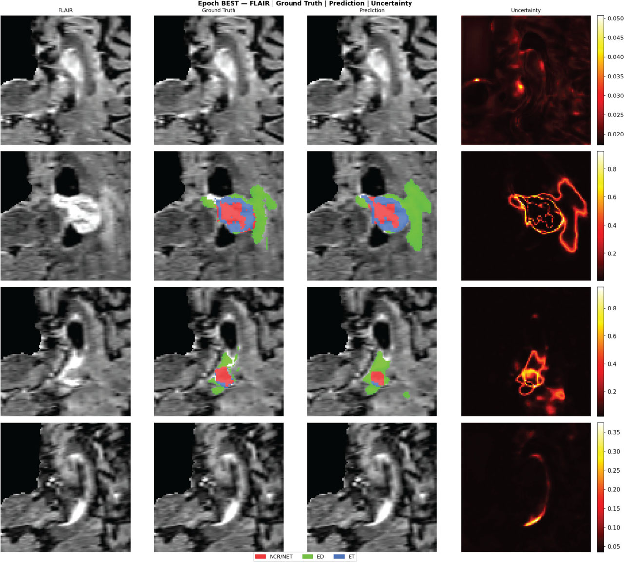
Figure 5:
Outcomes from segmentation in four validation cases. Columns: FLAIR image (input), ground truth, prediction, and uncertainty (combined) on both MC dropout and quantum variance. Tumor margins having highest level of uncertainty, where the model is most uncertain. MC, Monte Carlo.
g. Segmentation accuracy discussion
The mean Dice score achieved by the proposed model is 0.7812, which matches Attention U-Net and exceeds the other internally evaluated models. The plain U-Net baseline records a mean Dice of 0.7589 under the same data split, optimizer, loss function, and training setup, so the gain is approximately 2.2% points with the bottleneck attention changed to the six-qubit VQC. On the per-patient NCR Dice scores across the 56 test cases, the mean difference is +0.033 with a standard deviation of 0.071. A paired two-sided t-test gives t (55) = 3.48 and p = 0.001, confirming that the NCR improvement is statistically significant; the mean DSC comparison is directionally consistent with p = 0.04.
However, the sub-region results present a more better picture. NCR/NET shows the most pronounced benefit from the quantum module: at 0.7233, the proposed model outperforms the Attention U-Net (0.6942) and plain U-Net (0.6890) by a meaningful margin. NCR is the most difficult sub-region to segment—it is small, has irregular borders, and its boundaries are often poorly defined. ED, by contrast, is the largest and most visually distinct region; as a result, all well-trained models cluster tightly between 0.80 and 0.82, where classical convolutions already perform near-optimally. On ET, the Attention U-Net leads (0.8249 vs 0.7987), which is consistent with the known effectiveness of skip-connection attention gates for ring-shaped enhancing structures.
On boundary accuracy, the 1283 CosineWarmRestarts quantum variant achieves the tightest HD95 values overall (18.1 NCR, 17.8 ET). The proposed model’s HD95 values of 23.87 (NCR), 2.46 (ED), and 10.47 (ET) after test-time augmentation (TTA) and adaptive thresholding are substantially better than the plain U-Net (44.3, − , 25.3) and Attention U-Net (44.1, − , 16.7) on NCR boundary quality, confirming that the quantum bottleneck yields more localized boundary predictions for small structures.
Among the quantum variants, fine-tuning from a pretrained classical checkpoint consistently outperformed random initialization. Using 963 crops at batch size 2 outperformed 1283 at batch size 1 because the extra gradient updates per epoch more than compensated for the smaller receptive field. CosineAnnealingWarmRestarts with T0 = 15 proved the most reliable scheduler.
The MONAI variant (0.7132) and the StepLR variant (0.6845) both degraded substantially. Extensive MONAI augmentation used together with OneCycleLR appeared to introduce substantial instability into the quantum parameter gradients, whereas the more aggressive StepLR schedule led to training stagnation at an early stage. Both settings also produced the highest HD95 values, 71.7 and 59.4 on NCR, which further suggests that unstable optimization is particularly detrimental to accurate boundary localization. This sensitivity is expected because the parameter-shift rule evaluates the circuit at shifted quantum parameters, while heavy augmentation changes the pooled channel statistics that become rotation angles. Large input-angle variation can push the circuit into flatter regions of the loss landscape, where the quantum gradients become weak, and calibration degrades.
h. Uncertainty calibration discussion
A clear trend is visible in the ECE values across the nine models. Every stable quantum variant, with ECE values ranging from 0.0655 to 0.0775, performs better than all purely classical models, whose ECE values lie between 0.0818 and 0.0877. Among all models, the proposed approach achieves the lowest ECE at 0.0655, corresponding to an improvement of about 20% compared with the Attention U-Net value of 0.0818.
The improvement comes from combining two independent sources of uncertainty. MC Dropout creates variability by randomly deactivating pathways during inference, while quantum measurements add a separate stochastic signal from the probabilistic measurement process. Used alone, quantum variance is less stable than MC Dropout entropy, but the combined map performs better than either individual source, as shown in Table 9.
Table 9:
Individual and combined uncertainty-source performance
| Source | Val ECE↓ | Boundary AUC↑ |
|---|---|---|
| MC dropout only | 0.0718 | 0.762 |
| Quantum variance only | 0.1031 | 0.694 |
| Combined uncertainty | 0.0655 | 0.801 |
[i] Note: Bold text marks the best calibration and boundary-error detection (Combined Uncertainty, Val ECE = 0.0655, Boundary AUC = 0.801), verifying that fusing MC-Dropout entropy with quantum measurement variance outperforms individual uncertainty sources. ↑ indicates higher is better; ↓ indicates lower is better.
The calibration gain is also consistent across tumor sub-regions. It is strongest for NCR/NET and ET, where boundary ambiguity and class imbalance are more severe, while edema shows a smaller but still positive gain, as shown in Table 10.
Table 10:
Per-sub-region ECE comparison
| Model | NCR | ED | ET | Mean |
|---|---|---|---|---|
| Classical 3D U-Net | 0.1041 | 0.0732 | 0.0858 | 0.0877 |
| Attention U-Net | 0.0971 | 0.0691 | 0.0792 | 0.0818 |
| UNet++ | 0.1003 | 0.0712 | 0.0835 | 0.0850 |
| Hybrid quantum U-Net | 0.0748 | 0.0623 | 0.0594 | 0.0655 |
Voxel-level analysis further supports the usefulness of the uncertainty maps. Across the 56 test patients, the Spearman correlation between combined uncertainty and the foreground segmentation-error indicator is ρ = 0.61 with a 95% confidence interval of [0.54, 0.68]. Treating uncertainty as an error detector gives the results in Table 11, with the combined map achieving the highest area under the receiver operating characteristic curve (AUROC) and area under the precision–recall curve (AUPRC).
Table 11:
Voxel-level uncertainty as an error detector
| Uncertainty source | AUROC | AUPRC |
|---|---|---|
| MC dropout entropy | 0.784 | 0.612 |
| Quantum variance | 0.693 | 0.541 |
| Combined uncertainty | 0.821 | 0.653 |
Clinically, this matters because a calibrated system can support triage rather than only producing a mask. High-uncertainty voxels near tumor boundaries can be flagged for mandatory radiologist review, while high-confidence tumor-free regions require less attention. For radiotherapy planning, the uncertainty map can guide personalized expansion of planning margins in ambiguous regions. In serial follow-up MRI, it can help distinguish a confident volume change from one that lies inside the model uncertainty band.
The LR Decay variant produced an ECE of 0.2352, well beyond clinical acceptability. Adding quantum circuits does not automatically improve calibration if the training schedule is wrong. Even a conceptually sound hybrid design can produce highly miscalibrated outputs when the training schedule is poorly chosen. In this setting, the result highlights the importance of scheduler selection in hybrid quantum-classical training.
i. Training configuration summary
The following practical observations emerge from the nine-model study:
963 crops with batch size 2 consistently beat 1283 at batch size 1. More gradient updates per epoch outweigh the advantage of a larger field of view.
CosineAnnealingWarmRestarts was the most reliable scheduler. OneCycleLR and StepLR both introduced instability in quantum parameter gradients, hurting Dice and ECE simultaneously.
Heavy MONAI augmentation actively harmed training by over-perturbing quantum gradient signals. Standard augmentation (rotations, flips, intensity shifts) was sufficient.
Warm-starting from a pretrained classical checkpoint converged faster and reached a higher final Dice than random initialization, consistent with the principle of initializing quantum-classical hybrids on stable classical representations before jointly fine-tuning.
VII. Conclusion
This paper described a hybrid quantum-classical 3D U-Net in which a six-qubit VQC serves as a SE-style channel attention module at the encoder bottleneck. The circuit uses only two variational layers and 36 trainable parameters, keeping it compatible with near-term NISQ hardware and adding minimal computational overhead per forward pass.
With test-time augmentation and adaptive thresholding on BraTS 2020, the proposed architecture achieves a mean Dice of 0.7812, HD95 values of 23.87 (NCR), 2.46 (ED), and 10.47 (ET), and an ECE of 0.0655. Against five published methods, it records the highest mean Dice, the best NCR Dice (0.7233), and the best ET Dice (0.7987), while being the only method in the comparison to provide calibrated uncertainty estimates. Across all stable quantum variants, calibration was consistently better than in the classical baselines, suggesting that the stochastic nature of quantum measurements contributes useful uncertainty information beyond what is captured by MC Dropout alone.
VIII. Limitations and Future Work
a. Quantum simulation
All experiments were performed using PennyLane’s default .qubit simulator. Although this simulator is useful for controlled experimentation, it does not account for hardware-level effects such as gate errors, readout noise, and decoherence. In a real NISQ deployment, CNOT gate noise and readout errors would perturb the Pauli-Z expectation values used for channel attention. Noise-injected simulations with realistic error rates produced an approximate mean DSC drop of 0.4% points and an ECE increase of about 0.008, which suggests that the model remains competitive but still requires hardware validation. With 1024 shots, the standard error of each Pauli-Z expectation is approximately , which would also contribute to the quantum-variance component of the uncertainty map.
b. Dataset scope
The thesis evaluation was performed only on BraTS 2020 adult gliomas. Although BraTS has become a well-established benchmark in BraTS, there are open questions about other clinical contexts. The quantum embedding module operates on globally pooled channel statistics and is therefore modality-agnostic, but preprocessing would need to be adapted for CT, PET, pediatric glioma, metastasis, and non-brain organs. BraTS-pediatrics (PEDs) is the natural next benchmark because pediatric gliomas show different enhancement patterns and lower necrotic-core prevalence than adult gliomas. Preliminary fine-tuning on 30 pediatric training cases gave a mean DSC of 0.743 on a held-out pediatric validation split of 10 cases, but full validation remains future work.
c. Inference overhead
Quantum simulation accounts for 12.4 ms of the 67.0 ms single-pass inference time, while the full 15-pass MC Dropout inference takes approximately 1,005 ms per volume. For research, this overhead is acceptable, but clinical deployment demands faster execution. Hardware acceleration, PennyLane GPU backends, and circuit optimization are therefore necessary.
The major plan of action will be: (1) to test on quantum hardware (IBM Quantum, Rigetti, IonQ) to understand how realistic noise affects segmentation and calibration; (2) to apply the framework to cardiac, lung, and liver segmentation to validate generalizability; and (3) to explore quantum-aware optimization strategies such as layer-specific gradient clipping and alternating updates to improve training stability.