
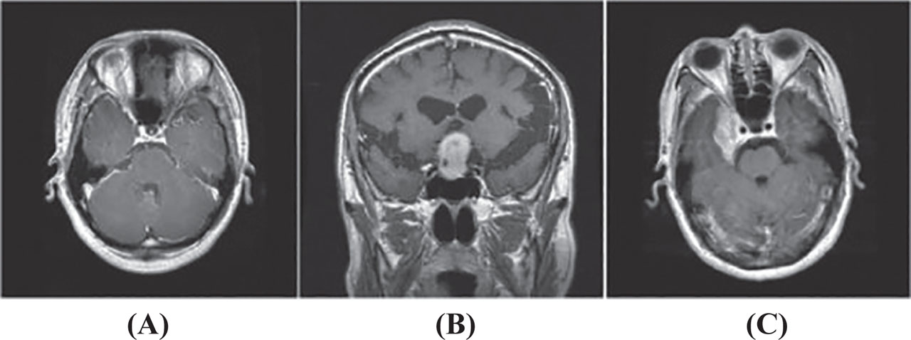
Figure 1:
Different categories of tumors: (A) glioma, (B) pituitary, (C) meningioma.
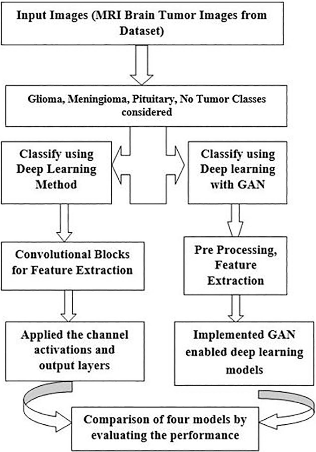
Figure 2:
Flowchart of the proposed framework. GAN, generative adversarial network.
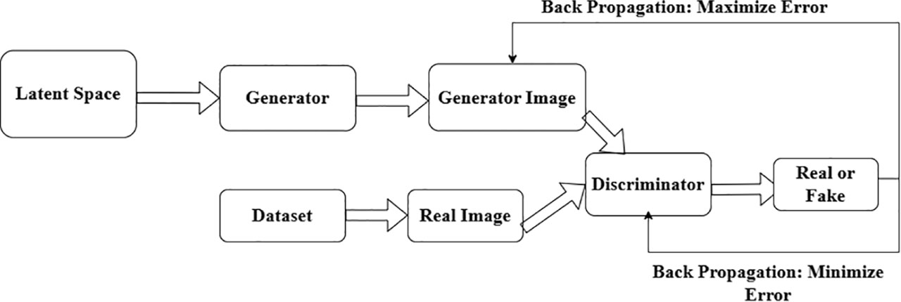
Figure 3:
GAN architecture showing generator and discriminator training process. GAN, generative adversarial network.
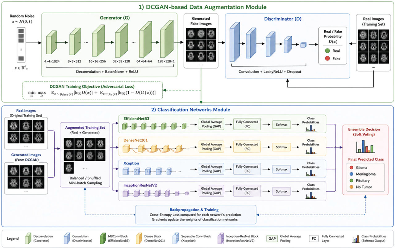
Figure 4:
Proposed DCGAN-based augmentation with classification networks. DCGAN, deep convolutional generative adversarial network; FC, fully connected; GAP, global average pooling.
Table 1:
Hyperparameter details
| Parameters | Value |
|---|---|
| Optimizer | Adam |
| Learning rate | 0.0002 |
| Batch size | 32 |
| Epochs (CNN) | 50 |
| Epochs (DCGAN) | 200 |
| Input size | 224 × 224 |
| Dropout | 0.6 |
| Activation | ReLU/LeakyReLU |
Table 2:
Performance analysis of models for brain tumor classification
| Model | Accuracy (%) | Precision (%) | Recall (%) | F1-score (%) |
|---|---|---|---|---|
| InceptionResNetV2 | 91.84 | 91.32 | 90.95 | 91.13 |
| Xception | 92.67 | 92.15 | 91.88 | 92.01 |
| DenseNet201 | 90.93 | 90.41 | 89.76 | 90.08 |
| EfficientNetB3 | 93.22 | 92.84 | 92.36 | 92.60 |
Table 3:
Fivefold cross-validation performance of the proposed EfficientNetB3 + DCGAN approach
| Fold | Accuracy (%) | Precision (%) | Recall (%) | F1-score (%) |
|---|---|---|---|---|
| 1 | 95.10 | 94.72 | 94.41 | 94.56 |
| 2 | 95.35 | 95.02 | 94.68 | 94.85 |
| 3 | 95.08 | 94.69 | 94.37 | 94.53 |
| 4 | 95.47 | 95.13 | 94.86 | 94.99 |
| 5 | 95.01 | 94.80 | 94.31 | 94.55 |
| Mean ± SD | 95.20 ± 0.19 | 94.87 ± 0.18 | 94.53 ± 0.22 | 94.70 ± 0.20 |
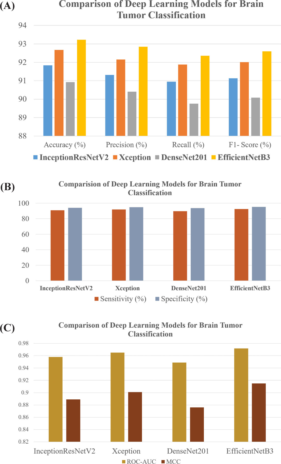
Figure 5:
Comparative analysis of models for brain tumor classification. (A) Comparison of accuracy, precision, recall and F1-score of the evaluated models. (B) Comparison of sensitivity, specificity. (C) Comparison of ROC-AUC and Matthews Correlation Coefficient (MCC).
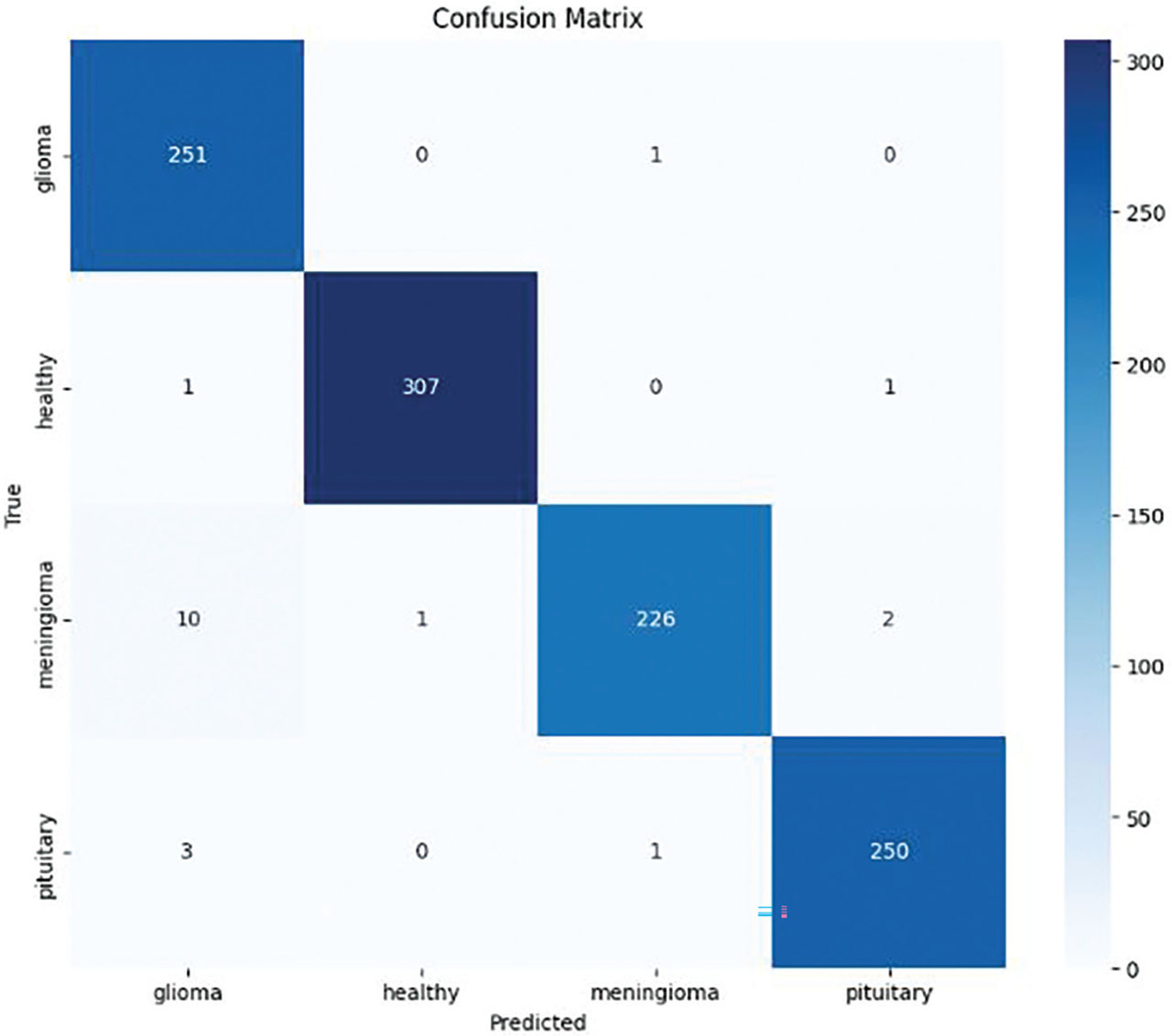
Figure 6:
Confusion matrix of the EfficientNetB3 model for multi-class tumor classification.
Table 4:
Performance analysis of DL models across various metrics
| Models | Sensitivity (%) | Specificity (%) | ROC-AUC | MCC |
|---|---|---|---|---|
| InceptionResNetV2 | 90.95 | 94.1 | 0.958 | 0.889 |
| Xception | 91.88 | 94.82 | 0.965 | 0.901 |
| DenseNet201 | 89.76 | 93.58 | 0.949 | 0.876 |
| EfficientNetB3 | 92.36 | 95.27 | 0.972 | 0.915 |
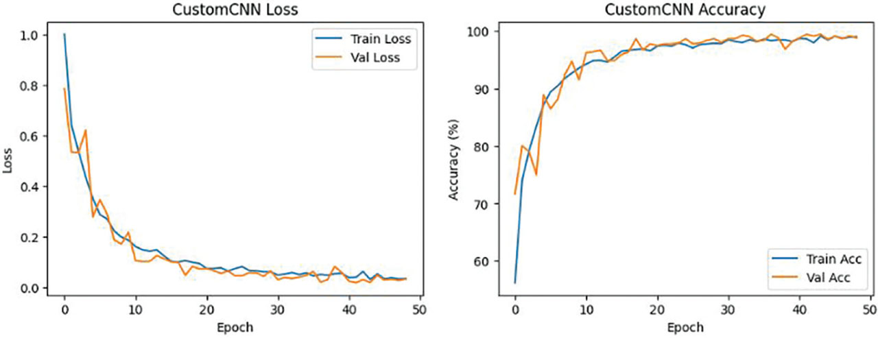
Figure 7:
Training and accuracy loss graph of the EfficientNetB3 model.
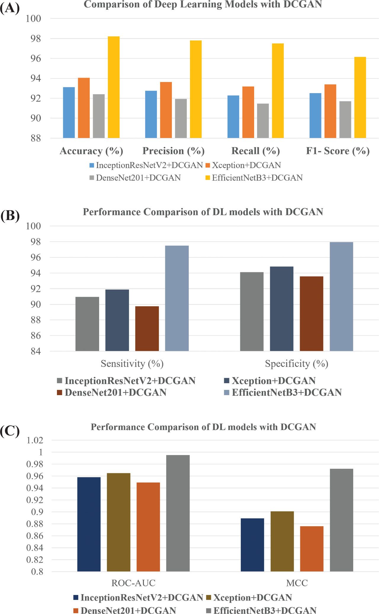
Figure 8:
Comparative performance analysis of DCGAN-integrated deep learning models. (A) Comparison of accuracy, precision, recall and F1-score. (B) Comparison of sensitivity, specificity. (C) ROC-AUC and Matthews Correlation Coefficient (MCC).
Table 5:
Performance of DL models with DCGAN for brain tumor classification
| Models + DCGAN | Accuracy (%) | Precision (%) | Recall (%) | F1-score (%) |
|---|---|---|---|---|
| InceptionResNetV2 + DCGAN | 93.74 | 93.28 | 92.94 | 93.11 |
| Xception + DCGAN | 94.58 | 94.12 | 93.76 | 93.94 |
| DenseNet201 + DCGAN | 92.86 | 92.33 | 91.95 | 92.14 |
| EfficientNetB3 + DCGAN | 95.20 | 94.87 | 94.52 | 94.69 |
Table 6:
Performance analysis of models across different metrics
| Models + DCGAN | Sensitivity (%) | Specificity (%) | ROC-AUC | MCC |
|---|---|---|---|---|
| InceptionResNetV2 + DCGAN | 92.94 | 95.68 | 0.973 | 0.918 |
| Xception + DCGAN | 93.76 | 96.21 | 0.981 | 0.932 |
| DenseNet201 + DCGAN | 91.95 | 95.07 | 0.967 | 0.901 |
| EfficientNetB3 + DCGAN | 94.52 | 97.14 | 0.989 | 0.956 |
Table 7:
Ablation study: Impact of augmentation strategies on EfficientNetB3 performance
| Model configuration | Accuracy (%) | Precision (%) | Recall %) | F1-score (%) |
|---|---|---|---|---|
| EfficientNetB3 (without augmentation) | 91.84 | 91.32 | 90.95 | 91.13 |
| EfficientNetB3 + Traditional augmentation | 93.22 | 92.84 | 92.36 | 92.60 |
| EfficientNetB3 + DCGAN augmentation | 95.20 | 94.87 | 94.52 | 94.69 |
Table 8:
Computational complexity analysis
| Model | Parameters (millions) | Training time (min/epoch) | GPU memory (GB) |
|---|---|---|---|
| InceptionResNetV2 | 55.9 | 5.8 | 9.6 |
| Xception | 22.9 | 4.7 | 8.1 |
| DenseNet201 | 20.2 | 4.1 | 7.5 |
| EfficientNetB3 | 12.0 | 3.8 | 6.9 |
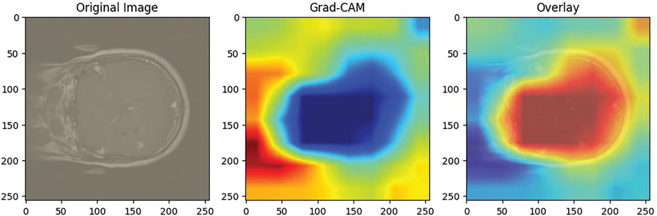
Figure 9:
Grad-CAM-based interpretability of the EfficientNetB3 model.
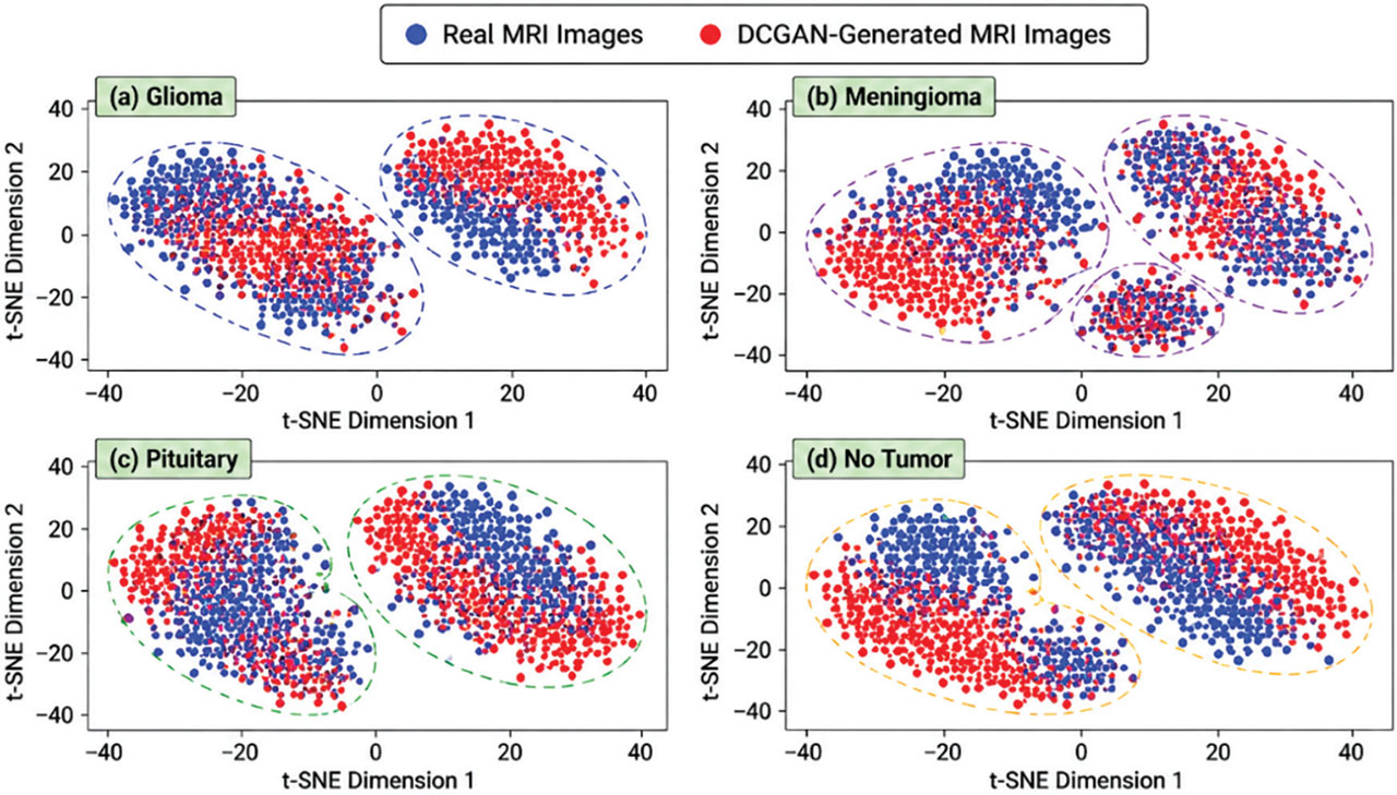
Figure 10:
t-SNE visualization comparing feature distributions of real and DCGAN-generated MRI images for multi-class brain tumor classification. DCGAN, deep convolutional generative adversarial network.
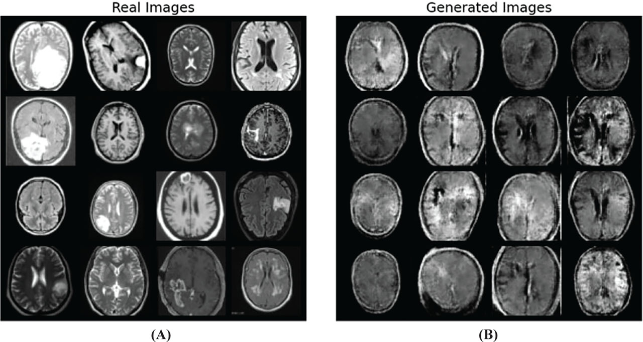
Figure 11:
Comparison of real and generated MRI images.
Table 9:
Comparative analysis of GAN models based on various metrics
| Model | FID | IS | SSIM | PSNR (dB) |
|---|---|---|---|---|
| Fully connected GAN | 165.8 | 1.92 ± 0.11 | 0.61 | 17.4 |
| Vanilla GAN | 124.6 | 2.45 ± 0.16 | 0.69 | 19.8 |
| DCGAN (proposed) | 72.3 | 3.81 ± 0.22 | 0.84 | 25.6 |
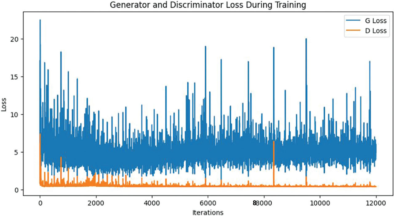
Figure 12:
Training loss curves of the generative and discriminative networks on the tumor dataset.
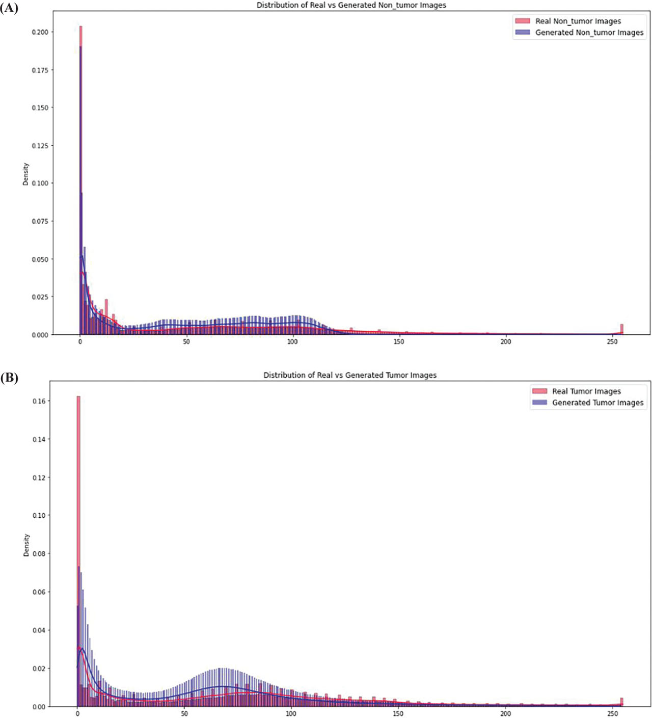
Figure 13:
Comparative analysis of density distribution between real and generated tumor and non-tumor images.