
I. Introduction
A malignant brain tumor derived from cerebral tissue can be life-threatening if left undetected. Medical experts often rely on MRI for accurate detection of tumors and high-resolution images. The primary brain tumors consist of several types: glioma, meningioma and pituitary adenoma. Pituitary tumors are high-grade malignant tumors that can cause serious neurological impairment. Deep learning (DL) models have achieved superior performance in brain tumor classification [1,2,3]. The advanced convolutional neural network (CNN)–based DL models enable research opportunities in tumor detection [4,5,6].
Generative adversarial networks (GANs) have recently become exceptionally efficient and strong-performing models in medical imaging, particularly when datasets are scarce and imbalanced. GANs are structured around two essential networks: a generator and a discriminator. The role of a generator is to generate synthetic MRI images, whereas the discriminator is responsible for differentiating real and synthetic images [7,8,9]. This approach facilitates the synthesis of high-quality tumor MRI images that improve data diversity and prevent overfitting in models. Compared with other cutting-edge GAN architectures, the deep convolutional GAN (DCGAN) is effective in diagnosing tumor-based classification MRI [10, 11]. In brain tumor classification, DCGAN-generated synthetic tumor images are incorporated with CNNs such as EfficientNetB3, DenseNet201, InceptionResNetV2 and Xception to enhance performance across glioma, meningioma and pituitary tumors. By augmenting training data and learning complex tumor patterns, GAN-based frameworks improve model performance and contribute to more accurate and efficient diagnosis of brain tumors [12, 13]. Figure 1 illustrates the various types of tumors. The early stage of diagnosis primarily focuses on observing the symptoms exhibited by patients with conditions affecting brain tissue [14].
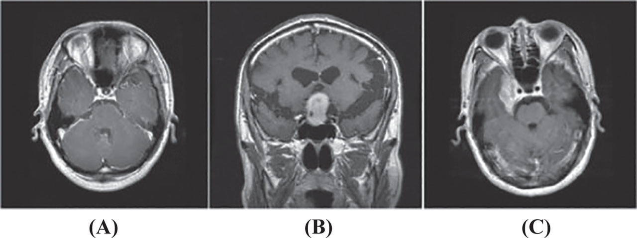
Figure 1:
Different categories of tumors: (A) glioma, (B) pituitary, (C) meningioma.
In recent years, the advancement of deep neural network models has enabled feature learning and enhanced accuracy for brain tumor classification, driving the widespread implementation of model architectures [15]. This study presents an innovative framework that integrates GANs with advanced neural network–based frameworks, including EfficientNetB3, InceptionResNetV2, Xception and DenseNet201, to achieve precise and early brain tumor detection. The structure of the current work is organized as follows: Section II demonstrates a comprehensive analysis of tumor detection and classification tasks employing DL models and DCGANs. Section III describes the methodology proposed in the present research, with a primary focus on the development of hybrid DL models integrated with DCGAN for feature enhancement and synthetic data generation. Section IV presents the experimental setup for brain tumor classification. Section V provides the results and discussion of the proposed models. Finally, the concluding section outlines the study and highlights potential directions for future research.
a. Research gap and motivation
Previous research primarily focus on deep CNN classification models or incorporate GANs for data augmentation. In contrast, limited focus has been provided on the systematic analysis of the quality of GAN-generated images and their effect on diagnostic performance under a standardized experimental setup. Furthermore, less attention is given to Grad-CAM-based visualization, which is crucial for clinical examination. The present study explores these shortcomings by combining GAN performance evaluation, comparative analysis of multiple models and AI interpretability techniques.
b. Contributions
The key findings of this study are summarized below:
A hybrid DL framework integrating DCGAN-based data augmentation with multiple state-of-the-art CNN architectures is proposed to address class imbalance in multi-class brain tumor classification.
Unlike existing studies that utilize GANs solely for image generation, this work leverages discriminator-driven feature refinement, enhancing representation learning within CNN models.
A comprehensive comparative analysis under controlled experimental conditions is conducted across four advanced architectures (EfficientNetB3, Xception, DenseNet201 and InceptionResNetV2).
DCGAN is preferred over GAN-based frameworks, including Wasserstein GAN (WGAN) and StyleGAN, because of its low computational cost and efficacy in MRI grayscale image synthesis under limited data-constrained conditions. The synthetic MRI images efficiently retained spatial and intensity-based tumor features, thus enhancing CNN generalization performance.
The study incorporates quantitative GAN evaluation metrics (Fréchet Inception Distance [FID], structural similarity index measure [SSIM], peak signal-to-noise ratio [PSNR], inception score [IS]) to validate the quality of synthetic MRI images—an aspect often overlooked in prior works.
Model interpretability is enhanced using Grad-CAM, providing clinically relevant visualization of tumor regions and improving trustworthiness in medical diagnosis.
II. Related Work
Brain tumor classification has emerged as a prominent research interest with various studies applying an advanced DL approach for medical image processing and analysis. Research professionals have proposed models for an accurate tumor diagnosis. GANs are extensively leveraged for synthetic image generation, thereby enhancing limited datasets. DCGANs are known for their potential to produce high-quality images in an unsupervised environment. Medical experts incorporated DCGANs to generate medical images for tumor classification.
a. Advanced DL models for brain tumor classification
DL models demonstrate promising results in improving efficiency for tumor classification, leading to enhanced diagnostic performance and the early detection of abnormal tumor patterns in medical images. The following section reviews research works on advanced DL methods for tumor analysis.
Peng and Liao [16] proposed a model that utilized image preprocessing and CNN techniques incorporated with the Adam optimizer. The results indicated an accuracy of 99.8% for the classification of tumors and demonstrated potential in the analysis of medical images.
Ayadi et al. [17] presented DL models for brain tumor classification. The model used in their study highlighted superior performance on datasets. The experimental results validate that the technique applied in their research was efficient compared to other existing methods.
Aziz et al. [18] developed the models for brain tumors with the DenseNet architecture. Transfer learning has been utilized using architectures involving DenseNet, ResNet, EfficientNet and MobileNet. DenseNet outperformed all other models by attaining the highest accuracy on the testing dataset. The authors applied hyperparameter tuning in their study for the most accurate results.
Pashaei et al. [19] designed a CNN-based architecture for feature extraction. The study reported an accuracy of 81%, which was further improved by an additional CNN classification model based on extreme learning machine. By examining classification discrepancies in pituitary and meningioma images, their study identified a limitation in the classifier’s capacity for discrimination.
Banerjee et al. [20] developed ConvNet and VGGNet models to process various MRI images. Their study explored the model’s performance and achieved an accuracy of 97% when tested on various MRI image datasets. A multilevel feature extraction technique was examined as a solution, which improved the model’s capacity to categorize brain tumors.
Ranjbarzadeh et al. [21] presented an efficient method for segmenting brain tumors. Their approach solved overfitting issues in a cascade DL model while reducing processing time. Furthermore, their results showed improvement in accuracy with the Dice score value generated (0.9203).
b. GAN-based augmentation
Recent research has demonstrated that deep feature extraction significantly enhances the performance of image classification and pattern recognition models, and transfer learning techniques in medical image analysis. GAN-based augmentation has achieved significant interest in brain tumor classification. Numerous research works have incorporated GAN models to generate real synthetic MRI images. The next section demonstrates research work on GAN for tumor-related image augmentation.
Afif et al. [22] developed synthetic images using DCGAN and incorporated them with real images in different proportions. Furthermore, a different real-world test set has been utilized to assess the CNN. Their results showed that when trained on synthetic data, the model performed well, providing robust sensitivity and precision for accurate tumor identification.
Irfan et al. [23] developed an advanced approach for detecting tumors by utilizing the power of generative models, such as WGAN and DCGAN. A strong CNN was used to examine the artificially improved images in order to precisely detect and categorize brain cancers. The comparison analysis showed how DL and synthetic image synthesis can be used to increase detection accuracy.
Chandana et al. [24] discussed the possibility of DCGANs to produce artificial brain tumor MRI images. The method used in their study demonstrated that DCGAN’s are effective in producing high-resolution grayscale images that replicate the characteristics and patterns of actual MRI scans. By artificially enriching the datasets, their work presented how DCGANs can be used to address the lack of medical imaging data, facilitating reliable diagnostic systems.
Mukherkjee et al. [25] developed three base GAN models: a WGAN and two variations of DCGAN. Additionally, the style transfer approach has been used to improve the image resemblance. The suggested model is able to generate high-quality images, with SSIM values of 0.57 and 0.83 across the respective datasets.
Chen et al. [26] enhanced the CNN performance with DCGAN by comparing the evaluation metrics. The classification accuracy of the model was determined based on the images containing meningioma, enhanced from 93.53% to 97.75%. Additionally, the F1 score showed significant improvement from 0.9187 to 0.9738.
Sandhiya et al. [27] employed DCGAN as a preprocessing strategy and compared it to other preprocessing methods. They employed Faster R-CNN to train the preprocessed data. Their work demonstrated high accuracy as compared to other CNN techniques, with the time taken for region proposal within 10 ms. Shyamala and MahaboobBasha [28] proposed DCGAN and CycleGAN for transforming images into different MRI modalities. Model generalization has been enhanced by incorporating GAN with CNN models. Moreover, DCGAN is effective for solving the data scarcity problem by generating artificial MRI images. The results of their work showed great results with a Dice score of 0.89, classification accuracy of 95.2% and FID score of 12.3.
Armoogum et al. [29] presented a transfer learning–driven classification model for breast cancer diagnosis and highlighted the significance of pretrained deep neural networks for enhanced generalization.
Ishrak et al. [30] introduced a transformer-based deep feature fusion system framework for the classification of keratoconus disease, suggesting the increasing adoption of hybrid DL approaches in medical imaging.
III. Proposed Methodology
The proposed work includes several steps as shown in Figure 2. These steps are discussed below.
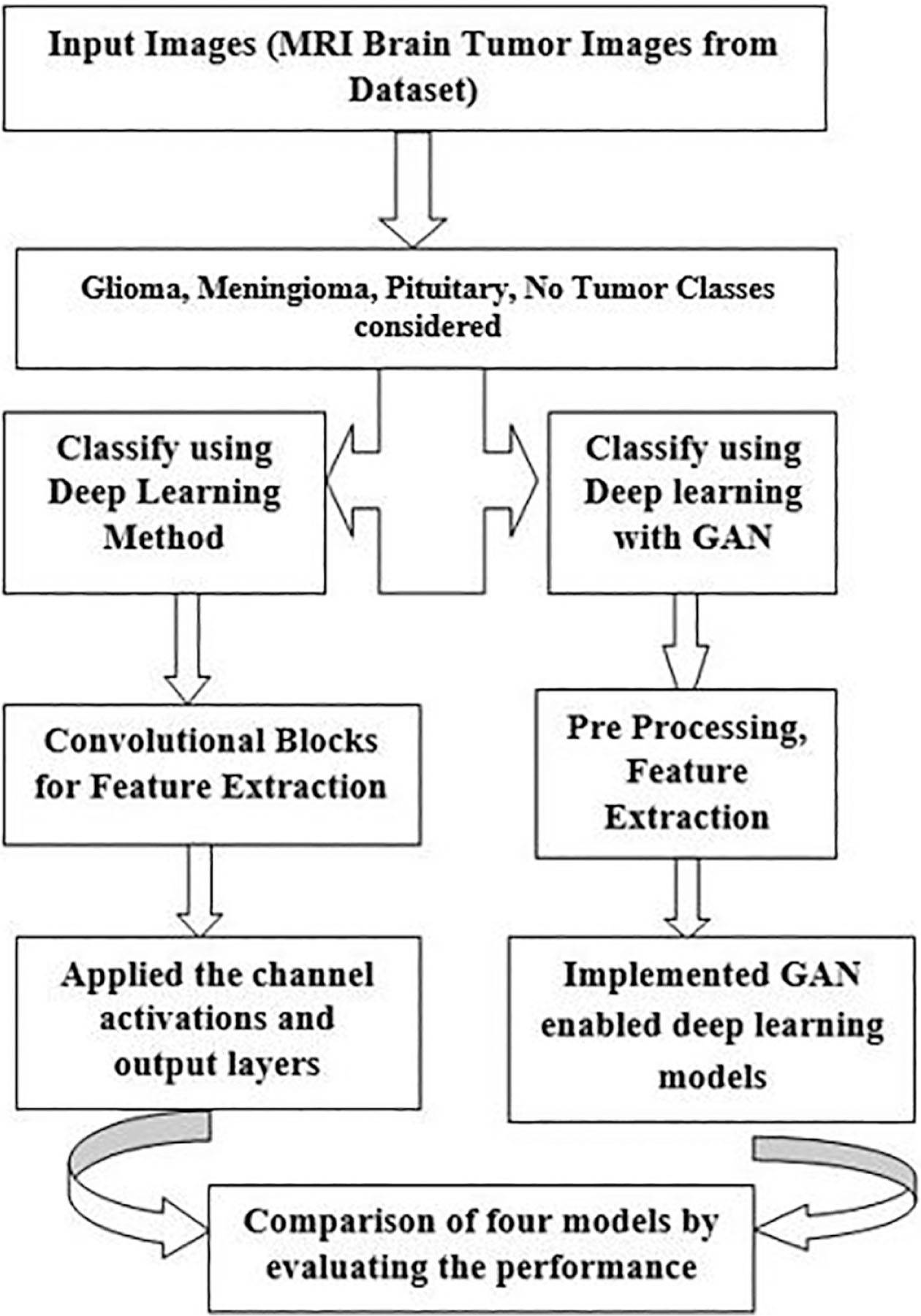
Figure 2:
Flowchart of the proposed framework. GAN, generative adversarial network.
Step 1: Input MRI Brain Tumor Images
The process starts with input MRI tumor images, which serve as the primary data source for the proposed model, capturing in-depth analysis of brain tissues. These images comprise multiple tumor classes, including glioma, meningioma, pituitary tumor and no-tumor. High-quality generated images are essential for improving the effectiveness and generalization ability of the model throughout the training process.
Step 2: Parallel Classification Framework
In this step, the MRI images are processed through DL classification models, where convolutional blocks learn and capture spatial and hierarchical feature representations. These extracted features are then utilized for accurate tumor classification. The GAN is then incorporated into the DL pipeline to produce synthetic images, which helps to handle class imbalance and enrich the training set, hence improving the classification model’s resilience.
Step 3: Convolutional Blocks for Feature Extraction (Without GAN)
Convolutional blocks are used to capture features from MRI images. Each block includes convolutional layers, activation functions and pooling operations that gradually learn spatial details such as edges, textures and tumor-related patterns. This layered feature extraction facilitates the model for accurate tumor classification.
Step 4: Channel Activation and Output Layers
Channel activation and output layers play an essential role in transforming learned features into final predictions using functions such as softmax for multi-class classification. The activation functions allow the model to capture complex feature representations, whereas the output layer transforms these learned features into the corresponding target class predictions.
Step 5: GAN-Enabled DL Model Implementation
The implementation of a GAN-assisted DL model combines GANs with traditional DL frameworks to boost overall performance. By producing realistic synthetic images, the GAN increases dataset diversity. This integrated strategy enables better feature extraction and ultimately enhances classification results.
The GAN model architecture and workflow are shown in Figure 3. First, the generator takes input from a low-dimensional latent space and learns to transform it into synthetic images. These generated images are intended to resemble real samples drawn from the original dataset. In contrast, real images originate from a high-dimensional sample space and contain structural and visual information. Both real and generated images are input to the discriminator network, which is trained to differentiate between authentic and synthetic images.
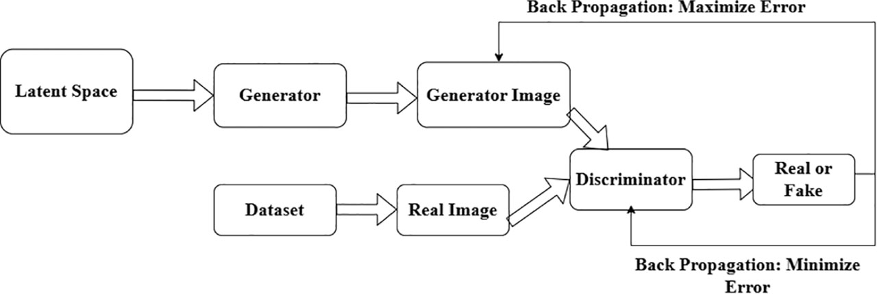
Figure 3:
GAN architecture showing generator and discriminator training process. GAN, generative adversarial network.
a. GAN objective function
The GAN objective function is shown in Eq. (1). GANs are formulated as a minimax game in which the generator attempts to fool the discriminator, while the discriminator aims to distinguish between real and synthetic data. The generator produces synthetic MRI images, whereas the discriminator learns to differentiate between real and generated MRI images.
x: Real MRI image
z: Random noise vector
b. Generator loss
The generator loss is shown in Eq. (2). It is designed to maximize the probability of the discriminator classifying generated samples as real. In other words, it aims to maximize log(D(G(z))), thereby encouraging the generator to produce data that is indistinguishable from real samples.
c. Discriminator loss
The discriminator loss is shown in Eq. (3), designed to train the discriminator network to accurately distinguish between real MRI images and synthetic images generated by the DCGAN.
d. Convolution operation (DCGAN)
The convolution operation is shown in Eq. (4), which evaluates feature maps by employing filters over the input, adding weighted values with bias and then followed by activation.
Step 6: Model Performance Evaluation and Comparison
The final step focuses on how accurately different models perform using performance metrics. By analyzing their results under identical settings, it becomes easier to determine which model works best. This analysis demonstrates the advantages and shortcomings of each method.
IV. Experimental Setup
This section provides the procedure followed to conduct the experiments and validate the proposed approach. It explains the dataset preparation process, training and testing the models, and the synthetic images generated using DCGAN. The evaluation process compares the efficacy of models for the multi-class brain tumor classification.
a. Dataset description
The dataset used in this work is obtained from the publicly available Figshare repository of brain tumor MRI images, comprising 7,023 MRI images, divided into four classes: 1,621 glioma cases, 1,645 meningioma, 1,757 pituitary and 2,000 no-tumor. The dataset is structured into training, validation and testing sets, where the training set is applied for training the model, the validation dataset for fine-tuning model hyperparameters and the testing set for final evaluation of model performance. To achieve the robustness of the evaluated performance, well-defined dataset partitioning (70% training, 15% validation and 15% testing) is maintained, preventing data leakage. A series of preprocessing steps is being done, which involves image resizing, data cleaning, noise reduction and data augmentation to develop a robust approach for brain tumor classification. The performance criteria incorporated metrics, including accuracy, precision, recall, specificity, F1-score, sensitivity, ROC-AUC and Matthews correlation coefficient (MCC). Thereby, strict image-level dataset partitioning is utilized to avoid potential data leakage.
b. MRI preprocessing pipeline
The traditional data augmentation strategies featuring horizontal flipping, rotation, zooming and brightness adjustment are incorporated alongside GAN-generated synthetic augmentation. Skull stripping and advanced denoising operations are not applied due to the already preprocessed nature of the public dataset.
c. DCGAN-based augmentation approach
The proposed architecture workflow is illustrated in Figure 4. It mainly consists of two major components: a DCGAN-based data augmentation module and a DL classification module. Initially, real MRI brain tumor images are provided to the DCGAN, where the generator creates realistic synthetic MRI samples from random noise vectors, whereas the discriminator evaluates their authenticity by distinguishing generated images from real images. By leveraging adversarial training, the generator is able to synthesize realistic MRI images with high visual fidelity, closely resembling authentic brain tumor scans.
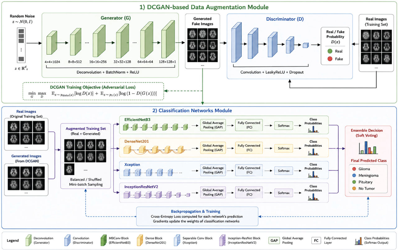
Figure 4:
Proposed DCGAN-based augmentation with classification networks. DCGAN, deep convolutional generative adversarial network; FC, fully connected; GAP, global average pooling.
The generated synthetic MRI images are incorporated with the original brain MRI dataset to generate a GAN-augmented training dataset. The enhanced dataset is utilized to train various CNN architectures such as EfficientNetB3, DenseNet201, Xception and InceptionResNetV2. Each network extracts discriminative tumor features and produces class probability predictions through fully connected and softmax layers. Finally, the outputs from all classification networks are integrated to generate the final tumor classification result. By increasing data diversity and reducing class imbalance, the DCGAN-based augmentation strategy enhances feature learning, improves model generalization and contributes to more accurate brain tumor classification.
d. DCGAN architecture and training
An evaluation is conducted on the quality of MRI images synthesized by the DCGAN model using both qualitative and quantitative evaluation metrics, including FID, SSIM, PSNR and IS. Training is continued until the generated images demonstrate anatomically meaningful tumor structures with minimal visual artifacts and stable generator-discriminator losses. Additionally, FID reduction and stable SSIM values are used as indicators of convergence and synthetic image realism prior to incorporating generated images into classifier training.
d.i. Mode collapse prevention strategy
To mitigate mode collapse, the following strategies are employed:
Adam optimizer with beta1 = 0.5 to dampen oscillations.
Batch normalization in generator layers to stabilize training.
One-sided label smoothing (real labels set to 0.9 instead of 1.0).
Periodic monitoring of the IS to detect diversity degradation.
The final IS of 3.81 ± 0.22 demonstrates that the generated images reflect significant diversity across tumor classes.
e. Model evaluation metrics
The performance of each model is quantified using the following metrics mentioned in Eqs (5)–(8), where TP indicates true positive, TN represents true negative, FP corresponds to false positive and FN denotes false negative.
f. Hyperparameter selection and optimization
The hyperparameters for both CNN and DCGAN training, as presented in Table 1, are selected based on repeated experimental evaluations and training convergence stability. The Adam optimizer is selected for its adaptive learning rate properties and reliable convergence in DL applications. An initial learning rate of 0.0002 is selected for DCGAN training to maintain stable adversarial learning dynamics while minimizing generator-discriminator imbalance. Batch size is selected according to available GPU memory and computational resources while preserving stable gradient updates. Dropout regularization and batch normalization layers are incorporated to reduce overfitting and improve model generalization. Adam optimizer is chosen due to its effective learning adaptability and stability in complex DL optimization problems. A momentum value of 0.5 is applied for stable GAN training. Batch sizes of 32, 64 and 128 are used based on GPU memory capacity and computing resources. A dropout rate of 0.6 is utilized to prevent overfitting issues and optimize generalization capability. The total number of epochs is maintained at 50 for CNN models, whereas DCGAN training is conducted for 200 epochs to ensure stable synthetic image generation. Training is performed till the generated MRI images achieve stable morphological structures with minimal imaging distortions and the GAN optimization losses attain stable convergence. To prevent mode collapse throughout the GAN training process, batch normalization and dropout-based regularization methods are utilized. The generator and discriminator loss values have been regularly monitored to ensure robust training behavior.
Table 1:
Hyperparameter details
| Parameters | Value |
|---|---|
| Optimizer | Adam |
| Learning rate | 0.0002 |
| Batch size | 32 |
| Epochs (CNN) | 50 |
| Epochs (DCGAN) | 200 |
| Input size | 224 × 224 |
| Dropout | 0.6 |
| Activation | ReLU/LeakyReLU |
Across all CNN architectures, the final classification layer is replaced with a task-specific classification module consisting of a global average pooling layer to reduce spatial dimensions, followed by a fully connected dense layer with 512 units and ReLU activation. A dropout layer (rate = 0.6) is applied for regularization, and the final dense layer contains four units with softmax activation to represent the four tumor classes. All models undergo initialization using ImageNet pretrained weights. Transfer learning is incorporated for deep convolutional models by employing ImageNet-based pretrained weights, which enhance training convergence and feature learning performance.
V. Results and Discussion
The following section presents a detailed discussion about the comparative analysis of DL models used for brain tumor classification. The experimental results demonstrate that GAN-based data augmentation enhances the robustness of CNN models for brain tumor classification. Additionally, GAN-driven augmentation increases feature variability and alleviates class imbalance, thereby improving model generalization without causing overfitting. Though GAN-based synthetic MRI augmentation considerably improved classification performance, it introduced additional computational overhead during training. The DCGAN training process utilized 200 epochs and high preprocessing time as compared to traditional augmentation techniques involving rotation and flipping. A performance comparison of DL models is provided in Table 2. Among the evaluated models, EfficientNetB3 achieved the highest performance, with an accuracy (93.22%), precision (92.84%), recall (92.36%) and an F1-score (92.60%). This indicates its effectiveness in correctly identifying tumor classes while maintaining a balanced trade-off between precision and recall.
Table 2:
Performance analysis of models for brain tumor classification
| Model | Accuracy (%) | Precision (%) | Recall (%) | F1-score (%) |
|---|---|---|---|---|
| InceptionResNetV2 | 91.84 | 91.32 | 90.95 | 91.13 |
| Xception | 92.67 | 92.15 | 91.88 | 92.01 |
| DenseNet201 | 90.93 | 90.41 | 89.76 | 90.08 |
| EfficientNetB3 | 93.22 | 92.84 | 92.36 | 92.60 |
EfficientNetB3 demonstrated better results than DenseNet201, Xception and InceptionResNetV2 models, mainly due to its compound scaling mechanism, which fine-tunes multidimensional scaling parameters more effectively than traditional CNN architectures. The architecture with balanced design facilitates enhanced feature extraction from complex tumor patterns in MRI images while ensuring minimized overfitting risk. In addition, EfficientNetB3 indicates robust compatibility with GAN-generated synthetic MRI images, leading to improved feature generalization capability among multi-class tumor classification categories.
To comprehensively evaluate the robustness and generalization capability of the proposed approach, fivefold cross-validation is performed for the EfficientNetB3 model integrated with DCGAN-based data augmentation. The average performance across the five folds is presented in Table 3, demonstrating the stability and reliability of the proposed work under different data partitions. The model indicates stable performance across all folds with slight variations in accuracy, demonstrating that the evaluation results are stable and not dependent on a specific train–test split.
Table 3:
Fivefold cross-validation performance of the proposed EfficientNetB3 + DCGAN approach
| Fold | Accuracy (%) | Precision (%) | Recall (%) | F1-score (%) |
|---|---|---|---|---|
| 1 | 95.10 | 94.72 | 94.41 | 94.56 |
| 2 | 95.35 | 95.02 | 94.68 | 94.85 |
| 3 | 95.08 | 94.69 | 94.37 | 94.53 |
| 4 | 95.47 | 95.13 | 94.86 | 94.99 |
| 5 | 95.01 | 94.80 | 94.31 | 94.55 |
| Mean ± SD | 95.20 ± 0.19 | 94.87 ± 0.18 | 94.53 ± 0.22 | 94.70 ± 0.20 |
a. Computational overhead and training efficiency
The incorporation of DCGAN-driven data augmentation led to an additional computational overhead compared with conventional approaches due to the adversarial training dynamics essential for MRI image synthesis. The DCGAN model training is performed over 200 epochs before achieving stable image quality. After synthetic MRI images were generated, the classifier training process remained computationally efficient due to the CNN models leveraging transfer learning with ImageNet-pretrained weights. Across the compared architectures, EfficientNetB3 exhibited lower computational cost and GPU memory usage while achieving superior classification performance, resulting in better efficiency of model training compared to more complex architectures such as InceptionResNetV2 and DenseNet201. Figure 5 illustrates a comparative performance analysis of DL models for tumor classification using various performance metrics. EfficientNetB3 achieved the highest accuracy across other evaluated models with less overfitting, suggesting its capability in extracting complex feature representations from MRI data. However, InceptionResNetV2 and Xception models also performed well, yielding robust results. In contrast, DenseNet201 demonstrated relatively lower accuracy in learning strong discriminative tumor patterns.
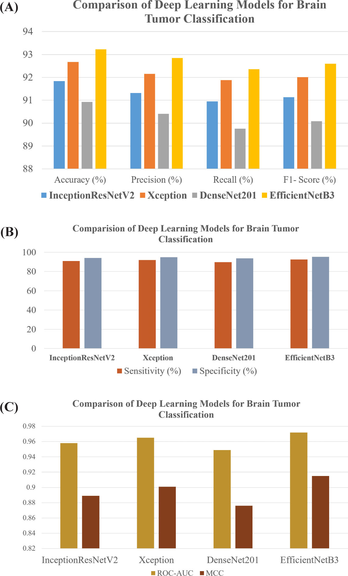
Figure 5:
Comparative analysis of models for brain tumor classification. (A) Comparison of accuracy, precision, recall and F1-score of the evaluated models. (B) Comparison of sensitivity, specificity. (C) Comparison of ROC-AUC and Matthews Correlation Coefficient (MCC).
The confusion matrix depicted in Figure 6 demonstrates the classification performance of the EfficientNetB3 model across four classes: glioma, healthy, meningioma and pituitary tumors. The results indicate robust class-wise performance, with the model accurately distinguishing among the different tumor categories and healthy brain images while exhibiting minimal misclassification.
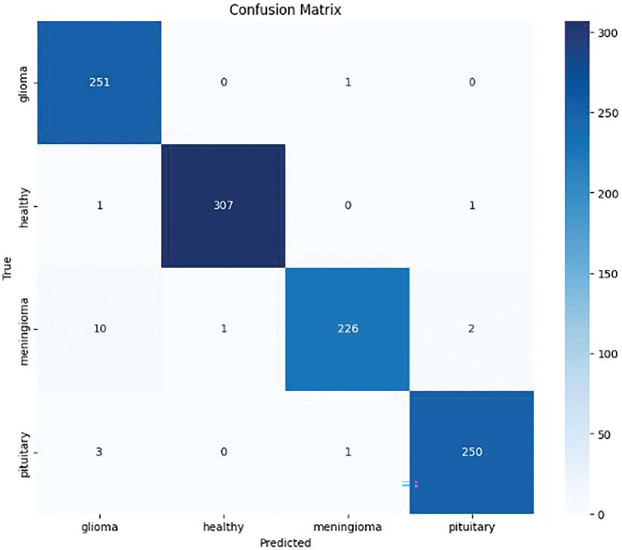
Figure 6:
Confusion matrix of the EfficientNetB3 model for multi-class tumor classification.
b. Misclassification analysis
The evaluation of misclassified MRI images demonstrates that classification ambiguity is identified between glioma and meningioma classes in low-intensity contrast MRI slices and initial-stage tumor findings where tumor boundaries exhibit visual indistinctness. Some incorrectly classified samples also include diverse tumor patterns and overlapping anatomical regions that diminish discriminative feature quality. In spite of these constraints, the presented EfficientNetB3-DCGAN model maintains robust discriminative capability across tumor types, suggesting effective feature extraction performance under complex radiological conditions.
c. Performance analysis of proposed models
The performance analysis of models is presented in Table 4, based on sensitivity, specificity, ROC-AUC and MCC. With the highest sensitivity (92.36%), specificity (95.27%), ROC-AUC (0.972) and MCC (0.915) of all the models, EfficientNetB3 exhibits the best performance. However, Xception yields satisfactory outcomes, followed by InceptionResNetV2, which demonstrates slightly lower sensitivity. DenseNet201 performs the lowest across all the metrics.
Table 4:
Performance analysis of DL models across various metrics
| Models | Sensitivity (%) | Specificity (%) | ROC-AUC | MCC |
|---|---|---|---|---|
| InceptionResNetV2 | 90.95 | 94.1 | 0.958 | 0.889 |
| Xception | 91.88 | 94.82 | 0.965 | 0.901 |
| DenseNet201 | 89.76 | 93.58 | 0.949 | 0.876 |
| EfficientNetB3 | 92.36 | 95.27 | 0.972 | 0.915 |
The training loss and accuracy curves in Figure 7 indicate the efficiency of the EfficientNetB3 model for brain tumor classification. The graphs demonstrate that training accuracy gradually rises, whereas validation accuracy moderately decreases, suggesting slight overfitting. In contrast, training loss declines steadily, and validation loss exhibits variation, highlighting subtle overfitting.
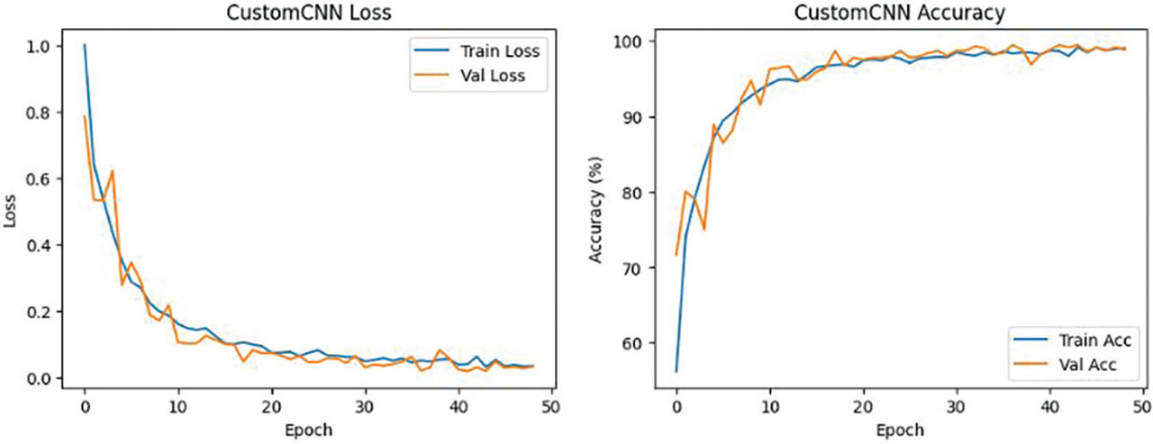
Figure 7:
Training and accuracy loss graph of the EfficientNetB3 model.
The performance analysis chart for DL architectures integrating with the DCGAN model is illustrated in Figures 8A–8C. In the first graph, evaluation metrics show consistently high values across models, with EfficientNetB3 demonstrating the best overall performance, followed closely by Xception and InceptionResNetV2. DenseNet201 exhibits slightly lower results but remains competitive. The second graph further supports these findings through sensitivity, specificity, ROC-AUC and MCC comparisons, where EfficientNetB3 again achieves superior scores, indicating better class discrimination and reliability. Thus, incorporating DCGAN improves model generalization, minimizes class imbalance and results in efficacy among models.
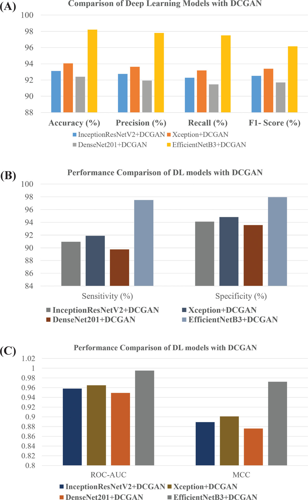
Figure 8:
Comparative performance analysis of DCGAN-integrated deep learning models. (A) Comparison of accuracy, precision, recall and F1-score. (B) Comparison of sensitivity, specificity. (C) ROC-AUC and Matthews Correlation Coefficient (MCC).
The comparative analysis for DCGAN-integrated models across evaluation metrics is shown in Tables 5 and 6. EfficientNetB3 incorporated with DCGAN outperforms the others, attaining the best classification accuracy (95.20%), with a sensitivity of 94.52%, specificity of 97.14%, ROC-AUC of 0.989 and an MCC of 0.956. However, the Xception and InceptionResNetV2 methods also demonstrate good performance across quantitative metrics. In comparison, DenseNet201 exhibits slightly lower performance results.
Table 5:
Performance of DL models with DCGAN for brain tumor classification
| Models + DCGAN | Accuracy (%) | Precision (%) | Recall (%) | F1-score (%) |
|---|---|---|---|---|
| InceptionResNetV2 + DCGAN | 93.74 | 93.28 | 92.94 | 93.11 |
| Xception + DCGAN | 94.58 | 94.12 | 93.76 | 93.94 |
| DenseNet201 + DCGAN | 92.86 | 92.33 | 91.95 | 92.14 |
| EfficientNetB3 + DCGAN | 95.20 | 94.87 | 94.52 | 94.69 |
Table 6:
Performance analysis of models across different metrics
| Models + DCGAN | Sensitivity (%) | Specificity (%) | ROC-AUC | MCC |
|---|---|---|---|---|
| InceptionResNetV2 + DCGAN | 92.94 | 95.68 | 0.973 | 0.918 |
| Xception + DCGAN | 93.76 | 96.21 | 0.981 | 0.932 |
| DenseNet201 + DCGAN | 91.95 | 95.07 | 0.967 | 0.901 |
| EfficientNetB3 + DCGAN | 94.52 | 97.14 | 0.989 | 0.956 |
Table 7 compares the performance analysis of EfficientNetB3 under various augmentation-based methods. The evaluation results demonstrate that DCGAN-driven augmentation yields superior classification performance with an accuracy of 95.20%, precision of 94.87%, recall of 94.52% and F1-score of 94.69%, outperforming both the baseline model and conventional augmentation techniques. This suggests the efficacy of DCGAN-synthesized images in improving classification performance for brain tumor diagnosis.
Table 7:
Ablation study: Impact of augmentation strategies on EfficientNetB3 performance
| Model configuration | Accuracy (%) | Precision (%) | Recall %) | F1-score (%) |
|---|---|---|---|---|
| EfficientNetB3 (without augmentation) | 91.84 | 91.32 | 90.95 | 91.13 |
| EfficientNetB3 + Traditional augmentation | 93.22 | 92.84 | 92.36 | 92.60 |
| EfficientNetB3 + DCGAN augmentation | 95.20 | 94.87 | 94.52 | 94.69 |
The computational complexity of the performed experimental evaluation of DL models is systematically compared in Table 8 on the basis of the number of parameters, training time per epoch and GPU memory consumption. Among the compared architectures, EfficientNetB3 delivers the best computational efficiency, utilizing the fewest parameters (12.0 million), the lowest training time (3.8 min/epoch) and the minimum GPU memory consumption (6.9 GB). In contrast, InceptionResNetV2 shows the highest computational overhead, with 55.9 million parameters and 9.6 GB of GPU memory usage. The findings highlight the efficient performance of EfficientNetB3 for MRI-based brain tumor classification.
d. Grad-CAM–based model interpretability analysis
The interpretability of the EfficientNetB3 model using Grad-CAM visualization is illustrated in Figure 9. To strengthen clinical decision-support interpretability, Grad-CAM-based visualization is embedded within the proposed architecture to localize tumor regions, facilitating most critical to the classification outcomes. The generated Grad-CAM heatmaps indicate that the deep CNN models mainly focused on diagnostically significant tumor boundaries and abnormal tissue areas instead of nontarget background structures. The model focuses on a localized region within the brain, which likely corresponds to the tumor-affected area. The concentrated red region in the heat map suggests that the model has successfully learned to identify meaningful pathological features rather than relying on irrelevant background information. Such interpretability mechanisms can assist radiology experts in analyzing model behavior and boost trust in AI-enabled diagnosis decisions.
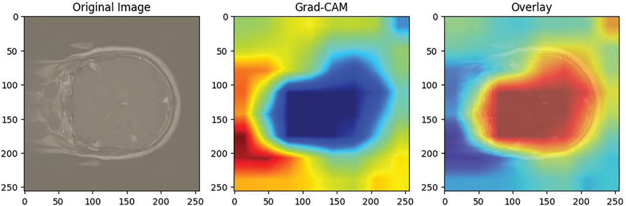
Figure 9:
Grad-CAM-based interpretability of the EfficientNetB3 model.
e. T-SNE visualization of real and synthetic MRI features
To analyze the quality and heterogeneity of the synthetic MRI images, t-SNE-based visualization is carried out on embedded feature vectors derived from real and DCGAN-generated MRI images. The analysis is performed to explore whether the synthetic images maintain the latent feature distribution of real tumor MRI scans while providing adequate diversity for robust augmentation. The t-SNE projection illustrated in Figure 10 indicates a significant overlap between the feature distributions of real and synthetic MRI images among various tumor categories. The generated MRI images closely align with the intrinsic data manifold of the primary dataset, suggesting that the DCGAN effectively learned meaningful structural and intensity-specific tumor features. The similarity observed between the real and generated latent feature clusters reveals that the DCGAN-synthesized images are useful for enhancing the generalization performance of the CNN for brain tumor classification.
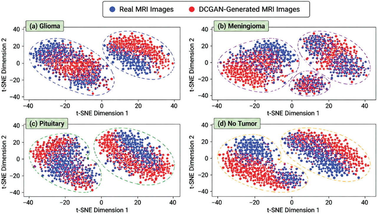
Figure 10:
t-SNE visualization comparing feature distributions of real and DCGAN-generated MRI images for multi-class brain tumor classification. DCGAN, deep convolutional generative adversarial network.
f. Synthetic data generation using DCGAN
DCGAN-based synthetic data generation involves training a generator-discriminator framework to produce high-quality synthetic images. The generator’s work is to generate images from random noise, whereas the discriminator performs an analysis of whether the images are real or generated. Through a continuous training process, the generator enhances its capability to generate real images. Moreover, DCGAN is extensively applied to enhance data scarcity by synthesizing high-quality images, which facilitates the improvement of model performance by preventing overfitting. Figure 10 shows the original MRI scans on the left, whereas the right panel displays synthetic images produced by the DCGAN model, highlighting its efficiency in generating realistic tumor patterns for data augmentation.
The performance of the generator and the discriminator is measured in terms of loss, shown in Figure 11. The findings demonstrate that the model performed well in generating realistic images for brain tumor classification. The generated MRI images exhibit notable diversity, and stable convergence behavior of generator–discriminator loss functions demonstrates that severe mode collapse is efficiently minimized throughout DCGAN training.
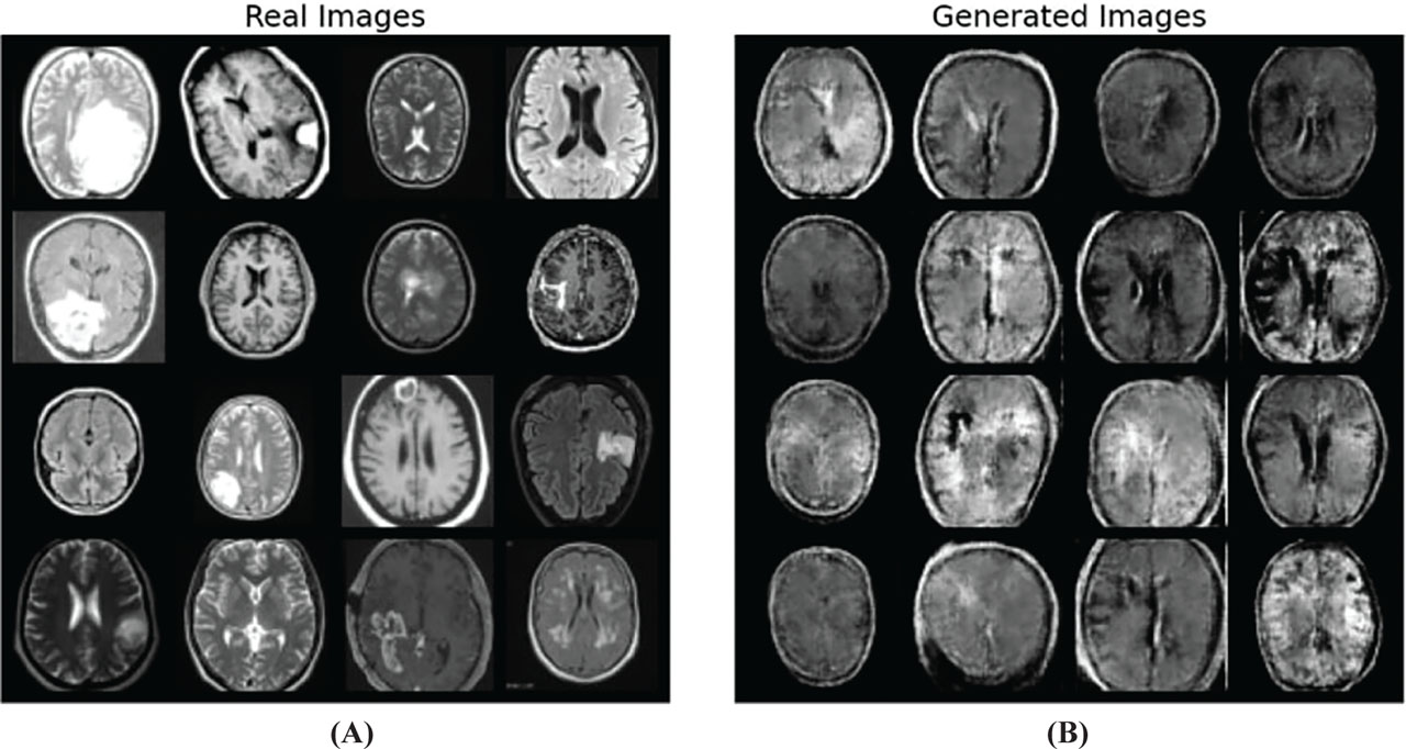
Figure 11:
Comparison of real and generated MRI images.
Furthermore, the performance of GAN models is provided in Table 9. With a high FID score of 165.8 and poor image quality performance parameters of (SSIM 0.61, PSNR 17.4 dB), the fully connected GAN had the lowest performance. By lowering the FID to 124.6 and improving image quality, the Vanilla GAN produced a more reliable output. With the lowest FID (72.3), highest IS (3.81 ± 0.22) and improved SSIM (0.84) and PSNR (25.6 dB), the suggested DCGAN performed the best, indicating better-quality generated images. The quantitative findings indicate that the synthetic MRI images attained satisfactory visual quality and structural similarity index, contributing to their use for training data augmentation.
Table 9:
Comparative analysis of GAN models based on various metrics
| Model | FID | IS | SSIM | PSNR (dB) |
|---|---|---|---|---|
| Fully connected GAN | 165.8 | 1.92 ± 0.11 | 0.61 | 17.4 |
| Vanilla GAN | 124.6 | 2.45 ± 0.16 | 0.69 | 19.8 |
| DCGAN (proposed) | 72.3 | 3.81 ± 0.22 | 0.84 | 25.6 |
The comparison between the distributions of real and synthetic images is shown in Figure 12, where the pixel intensity value is represented by x-axis and the image density is denoted by y-axis. In both scenarios, the pixel values are largely focused within the lower range, indicating that the generated images effectively maintain the critical intensity patterns of real non-tumor scans. The two curves consistent throughout the majority of the intensity spectrum indicate that the DCGAN model has successfully and minimally distorted the intrinsic data distribution. This demonstrates the performance of the DCGAN in synthesizing high-quality images.
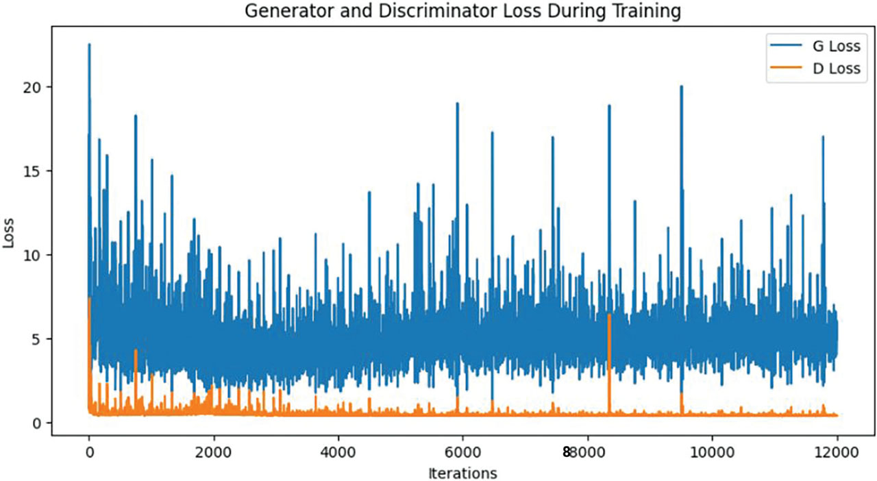
Figure 12:
Training loss curves of the generative and discriminative networks on the tumor dataset.
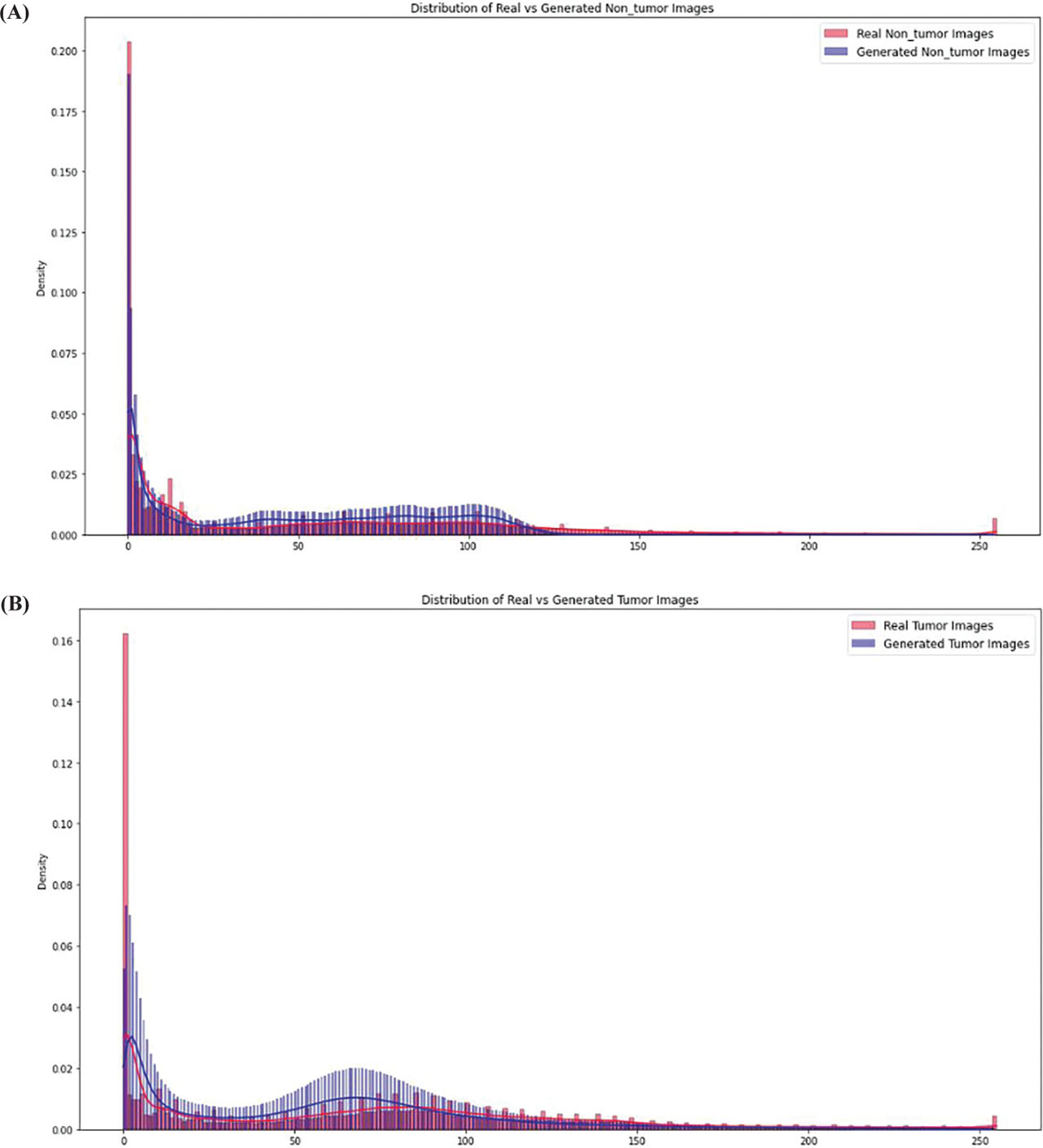
Figure 13:
Comparative analysis of density distribution between real and generated tumor and non-tumor images.
A performance comparison of different studies is presented in Table 10, based on the GAN models applied for data augmentation, the CNN backbone architecture utilized for classification and the obtained accuracy. The findings demonstrate that state-of-the-art CNN architectures integrated with GAN-driven data augmentation significantly strengthen tumor classification efficacy.
VI. Limitations
Although the proposed framework yields superior classification performance, the present work has certain limitations. First, the experiments have been performed on a publicly available dataset, which may affect the generalizability of the model across diverse imaging protocols. Second, GAN-driven augmentation employed additional processing overhead throughout the training process due to the generative adversarial image synthesis process. Furthermore, though MRI images generated by GANs enhanced classification accuracy, synthesized samples may exhibit subtle synthetic artifacts that can be challenging to detect through the use of evaluation metrics alone. However, Grad-CAM visualization optimizes explainable AI methods such as SHAP or attention-driven localization, which can further improve transparency in clinical decision-making.
VII. Conclusion
This study presents a DCGAN-driven DL framework for multi-class tumor classification using MRI images. The research work focused on two key challenges in automated diagnostic image analysis: data scarcity and class distribution imbalance in MRI datasets, and the need for high-performing, interpretable DL models capable of integration into clinical workflows. The quality of images generated by DCGAN is extensively analyzed using FID, SSIM, PSNR and IS, all of which showed significantly better results than the fully connected GAN and Vanilla GAN. The low FID score (72.3) and high SSIM value (0.84) validate that generated MRI images maintain the structural and intensity features of original clinical MRI scans, ensuring their suitability for robust data augmentation. Experimental findings across four advanced CNN models indicate that DCGAN-based augmentation enhances classification performance. The fusion of Grad-CAM-driven interpretability visualization yields clinically relevant evidence that EfficientNetB3 focuses on tumor-related anatomical areas instead of irrelevant background regions, therefore boosting model interpretability and improving reliability in AI-driven diagnosis. This interpretability framework is crucial for addressing the gap between DL models’ performance and clinical adoption.
Among the analyzed models, EfficientNetB3 integrated with DCGAN attained the best performance, demonstrating 95.20% accuracy, 94.87% precision, 94.52% recall and 94.69% F1-score. Furthermore, the ablation study demonstrates that GAN-based augmentation using DCGAN facilitates the greatest progressive performance improvement across both the baseline without data augmentation (91.84% accuracy) and the conventional augmentation pipeline (93.22%), establishing the essential role of synthetic data augmentation in the proposed approach.
Future work will explore UMAP-based feature embedding visualization to conduct a more detailed analysis of the feature overlap and variation between real and GAN-generated MRI image distributions. Additionally, GAN models, including WGAN, StyleGAN and diffusion-based generative frameworks, will be analyzed to strengthen the quality of synthetic MRI images.
Notes
[9] Data Availability and Reproducibility
To ensure reproducibility, the proposed work provides comprehensive details of the model architectures, preprocessing workflow, training setup and performance evaluation methodology. While the existing implementation and trained networks are not shared publicly, the experimental design has been discussed in-depth to facilitate future benchmarking studies and empirical validation.
[10] Conflicts of interest Conflict of Interest
The authors declare that this study was carried out without any commercial or financial affiliations that could be interpreted as constituting a potential conflict of interest.
[11] Publisher’s Note
The publisher remains impartial with respect to jurisdictional claims in published maps, institutional affiliations and any other geographical representations contained in this article. The opinions and conclusions presented are solely those of the authors and do not necessarily reflect the views of the publisher or the affiliated institutions.