
I. Introduction
In recent years, AI has experienced rapid growth in medical diagnostics, particularly in the fields of neurology and ophthalmology. Neurological and retinal illnesses are the leading causes of disability and vision loss globally, increasing the need for early, precise and efficient diagnostic techniques [1]. Traditional diagnostic approaches are practical yet time-consuming, require specialized interpretation and are challenging to access in distant or resource-limited areas [2]. Deep learning (DL), particularly convolutional neural networks (CNNs), can automate and enhance the identification of illnesses by analyzing complex medical imaging data [3]. Alzheimer's, Parkinson's and retinal diseases such as diabetic retinopathy (DR) and age-related macular degeneration are major public health issues. These illnesses require early detection to prevent progression and irreparable damage [4]. The heterogeneity of symptoms and imaging findings makes identification difficult. CNN-based systems can quickly and reliably classify segment and retinal anomalies by extracting and learning high-level features from massive datasets [5,6].
Neurological and ocular problems have increased worldwide, placing a strain on healthcare institutions to diagnose and treat them promptly [7]. Early stages of DR and neurodegenerative diseases such as Alzheimer's and Parkinson's progress silently, making traditional diagnostic methods less efficient at preventing long-term harm. Although many solutions are limited, machine learning (ML) and DL have been used in medical diagnosis [8]. They are difficult to deploy in remote or resource-constrained situations, and they must be understood and generalized across varied datasets. These constraints are particularly challenging in underdeveloped countries with limited medical competence and equipment [9].
This research proposes an integrated DL frame-work that utilizes high-resolution medical imaging data and advanced CNN architectures to detect retinal illnesses [10]. Transfer learning on pre-trained medical image classification models, such as ResNet50 and EfficientNet, improves diagnostic precision and speed [11]. The proposed system—transfer learning with pre-trained CNN models (TL-Pretr-CNN)—fine-tunes these models on massive and diverse datasets and utilizes explainable AI techniques, such as gradient-weighted class activation mapping (Grad-CAM), to provide clinicians with a visual explanation behind predictions [12].
Retina Vision Net, an integrated diagnostic frame-work using TL-Pretr-CNN such as ResNet50 and EfficientNet, addresses this issue [13]. These models are optimized for varied, high-resolution retinal disease detection, as discussed in Section 4. Grad-CAM visualizes predictions for clinical validation and decision-making [14,15].
Although numerous studies have applied DL to retinal disease detection, they face several persistent challenges: (i) poor generalization across multi-source retinal images due to variations in illumination, camera type and patient-specific pathology; (ii) limited interpretability, as most CNN-based models function as “black boxes,” reducing clinician trust; (iii) lack of integration with practical teleophthalmology workflows for real-time remote screening and (iv) difficulty in deploying computationally efficient models in resource-limited settings. These limitations restrict the clinical adoption of existing methods. To overcome these challenges, this study introduces TL-Pretr-CNN, a unified diagnostic framework that combines optimized transfer learning, enhanced preprocessing for cross-domain generalization and Grad-CAM–based visual explanations to ensure clinical transparency. Furthermore, the model's integration into a teleophthalmology system provides rapid, scalable and accessible screening support, distinguishing this research from previous DL approaches and establishing its significance in real-world health-care environments.
II. Related Work
a. DL techniques in medical imaging
Yang et al. [16] intended pre-trained CNN architectures—VGG16, DenseNet121, ResNet50 and ResNet152—for COVID-19 identification utilizing X-ray and CT-scan images. In CT-based binary classification, Fast. AI ResNet autonomously adjusted architecture, preprocessing and training to achieve over 96% accuracy and F1 score. In X-rays, enhanced VGG16 distinguished COVID-19 and pneumonia with 99% accuracy.
Rana and Bhushan [17] evaluate medical imaging-based ML and DL algorithms for illness identification and categorization. Experimental validation was performed on 40 primary studies using MRI datasets. DL models outperformed ML classifiers and CNN architectures in large medical datasets in terms of accuracy and scalability.
Wang et al. [18] offered a bibliometric study examining 2,685 original research articles from 2012 to 2020 to measure trends in medical image analysis DL. U-Net, ResNet, VGG and GANs were employed to segment and classify thoracic, abdominal and retinal scan datasets. Since 2017, DL applications have increased, with transfer learning dominating studies related to COVID-19.
Li et al. [19] examined medical image analysis using CNNs, RNNs, LSTMs, GANs and hybrid models. The study assesses algorithms on publicly available MRI, CT and X-ray datasets. CNNs are the most used approach, and Python is the chosen programming language. The accuracy and resilience of classification and segmentation tasks were often high.
The improved deep retinal intelligence detector network (IDRiD-Net) detects 16 retinal conditions from optical coherence tomography (OCT) images using a DL algorithm with uncertainty estimates, trained on massive, multi-device datasets, including internal and external test sets, as analyzed by Peng et al. [20]. It achieves an F1 score of up to 97.44% with a thresholding strategy and flags over 85% of nontarget or low-quality photos for manual review, outperforming state-of-the-art methods and human specialists.
Patel et al. [21] classified lung X-ray images using EfficientNet-B4 transfer learning and Grad-CAM for explainable multi-disease classification. We trained the model on a dataset of lung X-rays featuring COVID-19, pneumonia, tuberculosis and pulmonary nodules. Grad-CAM visuals improved interpretability and classification accuracy to 96%.
b. Retinal disease detection with CNNs
Sarah et al. [22] classified OCT images into diabetic macular edema, drusen and choroidal neovascularization using CNNs with various optimizers and regularization methods. The collection includes over 80,000 annotated retinal scans from Kaggle's OCT picture dataset. The model achieved a classification accuracy of over 98%, with high precision and recall.
Tayal et al. [23] introduced an OCT retinal scan–based DL diagnostic system utilizing CNNs with five, seven and nine layers to classify four ocular conditions: diabetic macular edema, drusen, choroidal neovascularization and normal retina. OCT images preprocessed for noise removal, contrast enhancement and contour identification are in the collection. The proposed models outperformed manual diagnosis in classification accuracy (96.5%), sensitivity (96.0%) and specificity (98.6%).
Diwan et al. [24] examined the You Only Look Once (YOLO) family of object detection models, which use regression-based formulations to recognize objects in a single network run. The study evaluated several YOLO variants on the COCO and PASCAL VOC datasets. The results showed that YOLO achieved up to 63.4% detection accuracy while providing inference speeds approximately 300 times faster than two-stage detectors such as Fast R-CNN, which achieved around 70% detection accuracy.
Valanarasu et al. [25] implemented KiU-Net, a dual-branch segmentation architecture, which uses an overcomplete network (Kite-Net) for fine details and U-Net for high-level feature learning. The suggested technique achieved strong segmentation with fewer parameters and faster convergence on five varied medical imaging datasets. The results revealed greater boundary precision and small structure recognition than typical U-Net variations. The KiU-Net 3D extension improved volumetric segmentation.
Despite significant progress in DL-based retinal disease detection, existing studies primarily focus on isolated CNN architectures, limited datasets and single-disease classification without addressing clinical interpretability and deployment challenges [26,27,28,29]. Most methods lack robust generalization across diverse imaging conditions, do not integrate explainable AI tools for clinician trust and are rarely designed with teleophthalmology support for use in remote healthcare environments. These gaps restrict scalability and limit their clinical applicability.
Unlike existing studies that focus on single-disease classification, limited datasets or non-explainable CNN models, this research introduces a unified and clinically oriented framework that combines optimized transfer learning, multilevel retinal disease grading and Grad-CAM–based interpretability. The proposed TL-Pretr-CNN model is designed to generalize effectively across heterogeneous high-resolution fundus images while providing transparent visual explanations to support clinical decision-making. This integrated approach, along with teleophthalmology compatibility, establishes a stronger practical contribution compared to prior literature and demonstrates the system's applicability in real-world healthcare environments.
III. Methodology
The TL-Pretr-CNN framework (Figure 1) uses DL to detect and classify DR using high-resolution fundus pictures. Image preprocessing improves quality and standardizes inputs. Basic layers are frozen through transfer learning, while top layers and a custom classification head are fine-tuned to extract deep features from pre-trained CNN models, such as ResNet50 and EfficientNet. These features let a classification layer assess DR severity (no, mild, moderate). Grad-CAM heatmaps highlight important locations that influence model predictions, thereby enhancing clinical transparency and accuracy. Teleophthalmology applications for remote screening and patient prioritization utilize data in a decision support system.
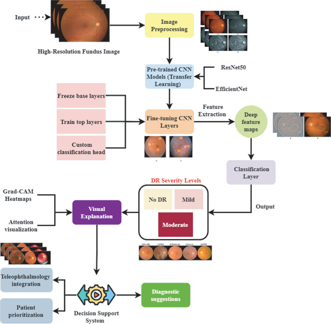
Figure 1:
TL-Pretr-CNN framework for automated retinal disease detection and classification. CNNs, convolutional neural networks; DR, diabetic retinopathy; Grad-CAM, gradient-weighted class activation mapping; TL-Pretr-CNN, transfer learning with pre-trained CNN models.
a. Data acquisition and preprocessing
The study utilizes a large-scale retinal fundus image dataset containing 130,993 images, each annotated with one of five DR severity levels: No DR, mild, moderate, severe and proliferative DR. This dataset is sourced from a publicly available benchmark repository widely used in DR classification research. The size discrepancy mentioned earlier was due to partial subsets being described during the preprocessing explanation; however, the complete dataset used for training, validation and testing consists of 130,993 images, which is consistently applied throughout the model development pipeline.
All images were captured using high-resolution fundus cameras under varying illumination and field-of-view conditions, reflecting real-world clinical variability. The dataset offers a balanced representation across DR stages, though mild class imbalance natu-rally exists in higher severity grades—typical of epidemiological DR distributions.
To mitigate the class imbalance, stratified sampling was employed to split the dataset into training (70%), validation (15%) and testing (15%) sets, ensuring proportional representation of all five DR classes in each subset. This preserves clinical representativeness and prevents bias during model optimization. In addition, data augmentation was applied preferentially to underrepresented classes, including contrast-limited adaptive histogram equalization (CLAHE)-based contrast enhancement, rotations (±20°), random cropping and brightness/contrast adjustments, to artificially balance the training data and improve generalization. While explicit k-fold cross-validation was not performed, the separate validation set was used for hyperparameter tuning and monitoring overfitting, and the final testing set provided an unbiased evaluation of model performance.
Each image, provided in RGB format with varying dimensions, was resized to a fixed resolution as part of preprocessing. Normalization, augmentation and contrast enhancement via CLAHE were applied as follows:
where Ii is the original image, μ and σ are the mean and standard deviation, Rθ applies rotation by θ, Fp performs flipping with probability p, Zs applies zoom by scale s and α is the CLAHE clip limit. This preprocessing pipeline ensures uniform intensity, improved lesion visibility and robust feature learning for subsequent CNN-based DR classification. Table 1 shows the preprocessing steps in retinal disease.


a.i. Normalization
Medical image analysis requires normalization to ensure a uniform pixel intensity distribution across all images. The formula is:
Here, in Eq. (1), Ii is the original pixel intensity, μ is the image's mean and σ is the standard deviation. This procedure reduces intensity-related variability by scaling the image data to have a mean of zero and a variance of one. Multimodal inputs, such as retinal images, benefit from faster neural network convergence and improved generalization across datasets.a.ii. Augmentation transformation function
The augmentation transformation function T is designed to artificially expand the training dataset by introducing variations, improving model robustness. It is defined as:
where in equation 2, Rθ applies a rotation to the image by an angle θ, Fp performs horizontal or vertical flipping with a probability p, Zs zooms the image by a scale factor s. These transformations simulate real-world variations in medical imaging, reducing overfitting and enhancing the model's ability to generalize to unseen data.a.iii. Contrast enhancement via CLAHE
For better visibility of retinal blood vessels and anatomical boundaries, Contrast Limited Adaptive Histogram Equalization (CLAHE) is applied to the normalized image, as expressed in Equation (3):
This equation contains the entire preparation workflow for retinal fundus images. Three crucial preprocessing operations are applied to each raw input image Ii from the dataset. The first step is to normalize pixel intensities by eliminating the mean (μ ) and dividing by the standard deviation ( σ ) to create the norm (Ii). Second, CLAHE improves local contrast by dispersing pixel intensities in adaptive tiles, controlled by the clip limit α, thereby enhancing the visibility of features such as blood arteries and tumor edges. Third, the augmentation function T includes rotation Rθ, flipping Fp and zooming Zs to boost model robustness and reduce overfitting. The fully normalized, extended and augmented dataset Ipre is optimized for deep CNN-based feature extraction and classification.
An initial convolution and max-pooling layer retrieves fundamental visual information from a 224 × 224 × 3 input image. Multiple residual blocks (Conv2–Conv5) extract hierarchical features as filter sizes increase, capturing increasingly abstract and complicated patterns. A global average pooling (GAP) layer reduces spatial redundancy by compressing feature maps into a 2,048-dimensional vector. Lastly, a fully connected layer enables reliable and interpretable disease classification for medical image diagnosis.
b. Feature extraction with transfer learning
In this research, transfer learning utilizing pre-trained CNN models, such as ResNet50 and EfficientNet, extracts disease-specific characteristics from retinal fundus data. These models, trained on ImageNet, have extensive feature extraction capabilities that are fine-tuned on medical datasets. The models can detect retinal microaneurysms by freezing lower layers and adjusting upper layers to domain-specific properties. This method reduces training time, enhances accuracy and leverages learned visual hierarchies to diagnose diseases in multimodal medical imaging.
b.i. Transfer learning with pre-trained CNN backbones (ResNet-50, EfficientNet-B0)
The TL-Pretr-CNN system uses ImageNet-trained backbones (ResNet50, EfficientNet) to grade DR. High-resolution fundus images undergo preprocessing, followed by the application of frozen foundation layers to maintain universal edge and texture detectors. The final convolutional block and a bespoke softmax head are fine-tuned on retinal input to reduce training costs and prevent overfitting. The original feature hierarchy is maintained while a limited parameter subset is updated using a unified loss (cross-entropy plus L2 regularization). GAP and Grad-CAM improve clinician trust by compressing spatial maps into a compact vector for categorization and highlighting lesion locations. Let a color fundus image be I ∈ ℝ224×224×3 after preprocessing. The components of a generic ImageNet network can be broken down into
In Equation (4), gbase denotes the stack of early and intermediate convolutional layers (e.g., ResBlocks in ResNet-50 or MBConv blocks in EfficientNet) that learn generic low-level features such as edges, textures, and shapes. ghead represents the high-level classification layers, including the global average pooling layer and the original 1,000-class softmax classifier.
a) Freezing the Generic Feature Extractor: To conserve universal visual filters, we freeze θbase from from Eq. (5):
To freeze transfer learning, block modifications to the generic feature extractor's weights (θbase). To preserve the generic visual features learned during pre-training, the parameters of the feature extraction backbone are frozen during training. This is achieved by setting the gradient of the training loss L with respect to the base network parameters θbase to zero
After training, the optimal base parameters , remain identical to the pre-trained ImageNet weights . Here, θbase denotes the parameters of the early and intermediate convolutional layers responsible for learning generic visual features such as edges, textures, and shapes. Freezing these layers allows the network to optimize only the task-specific classification layers, thereby reducing training time, minimizing the risk of overfitting on limited medical datasets, and leveraging robust feature representations learned from the large-scale ImageNet dataset.
b) DomainSpecific FineTuning: Utilize a custom DR classifier gcls with parameters θcls and adjust the last convolutional block gtop (e.g., Conv5_x in ResNet-50) from Eq. (6):
A medical image I is processed through the transferlearning network to yield a high-level feature map. The inner function gbase represents the frozen, generic feature extractor whose parameters are locked (equal to the ImageNet-trained values). It converts the input image into intermediate activations. These activations are then passed to gtop, the trainable adaptation block parameterized by θtop is fine-tuned on domain-specific data to capture pathological cues. The final output F is a tensor of spatial dimension 7 × 7 with d channels, encapsulating rich, task-aware visual descriptors that feed subsequent pooling or classification layers. Applying GAP yields from Eq. (7):
The d-dimensional activation vector at the spatial location (h,w) within the 7 × 7 feature map generated by the fine-tuned CNN is denoted by Fh,w ∈ Rd, where h and www represent the spatial coordinates and d is the number of feature channels. Summing all 49 location vectors and dividing by 49 yields the mean activation for each channel, keeping channel-wise semantics while reducing spatial dimensions. A compact d-length representation, z, contains the most important aggregated information from the full feature map. Reduced dimensionality prevents overfitting, integrates smoothly into fully connected or softmax layers and maintains the network's capacity to identify patterns across the image. The custom head maps z to the C DR grades (C = 3 in: noDR, mild, moderate) in Eq. (8):
where W ∈ ℝc×d and b ∈ ℝc are learnable parameters. Using GAP, the channel-wise feature vector obtained is z ∈ ℝ, . The linear transformation Wz+b converts pooled characteristics into a C-dimensional logit vector, where c represents the number of disease classes (e.g., DR severity levels). The softmax function translates logits into a probability distribution , where the ith component indicates the network's confidence in class i for the input image. The top layers (W and b) are trained end-to-end, while the GAP representation (z) ensures that spatially summarized, semantically rich information drives the classification choice.The pipeline begins with preprocessed fundus photos fed into a frozen ImageNet backbone (ResNet-50 or EfficientNet-B0), as illustrated in Figure 2. The locked parameters . As shown by the edge detection and feature enhancement responses, the frozen convolutional layers preserve edge and texture detectors learned during pre-training.
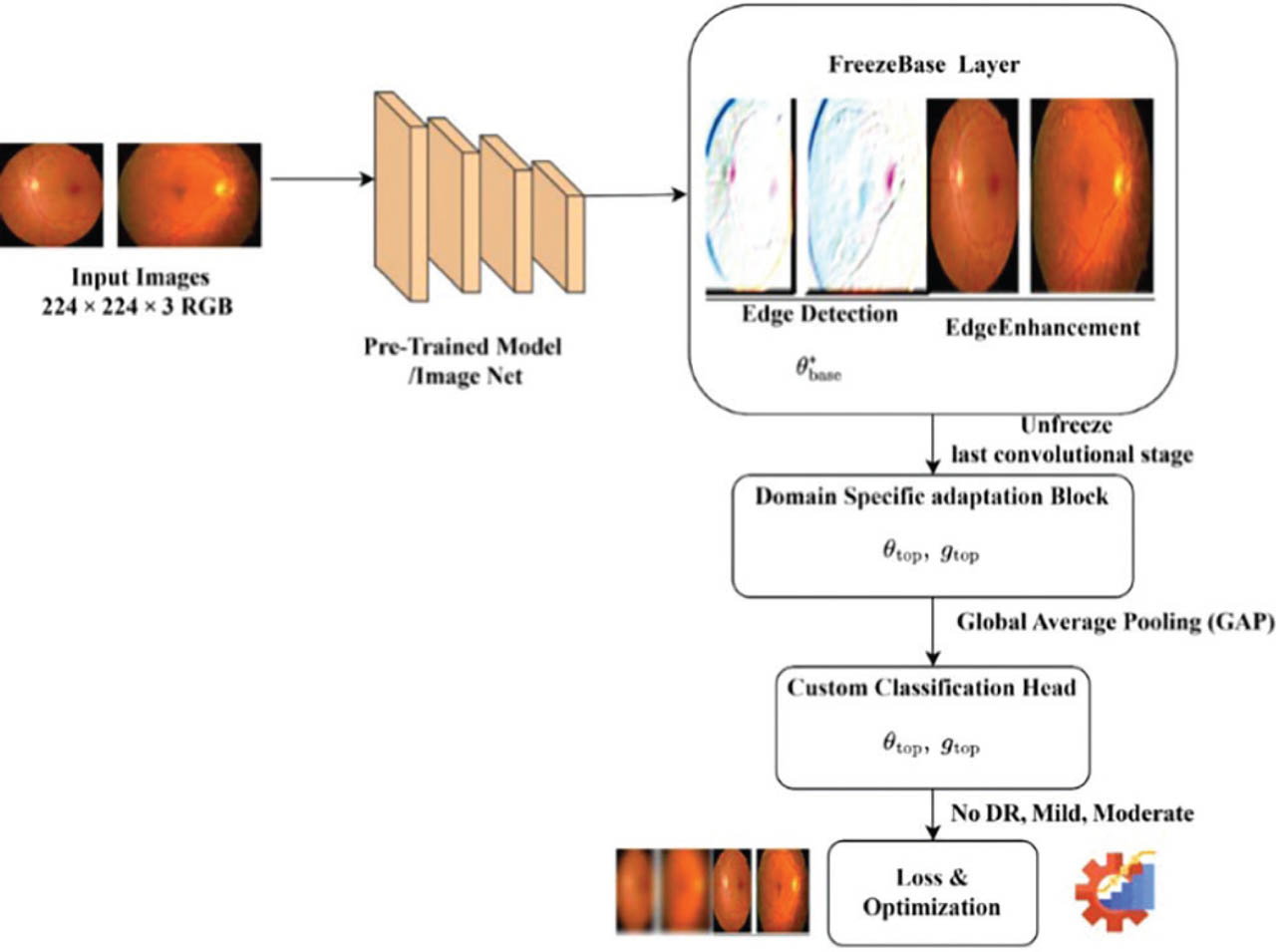
Figure 2:
TLPretrCNN workflow for multimodal retinal diagnosis. CNNs, convolutional neural networks; DR, diabetic retinopathy; GAP, global average pooling; TL-Pretr-CNN, transfer learning with pre-trained CNN models.
b.ii. Transfer learning optimization for medical images
The implied TL-Pretr-CNN, designed for combined MRI of the retina, is shown in the panel as it gradually improves visual evidence from generic edges to pathology-aware signs. It is illustrated in Figure 3. Four representations are sent to the network in the blue “Input Pattern” column: (a) the contrast-normalized image, (b) the edge map, (c) the fused pathological prior and (d) the Grad-CAM saliency seed. The most activated channels following each residual block (Conv2–Conv5) are shown in green columns, a–d. The ability of Conv2 (the frozen version of BaseNet) to respond to universal contours, such as optic disk rings and cranial outlines, shows that it has retained the primitives from ImageNet. As the partially trainable α head becomes more adaptive, Conv3 starts to specialize in tasks, retinal maps improve micro-aneurysm rims and MRI maps define ventricular borders. Fully trainable Conv4 ( θ top) enhances lesion-centric filters; activations with color coding identify tumor textures and hemorrhages, demonstrating domain transfer. The interpretability is validated when Conv5 feeds the custom softmax head; Grad-CAM overlays co-localize with clinically significant regions.
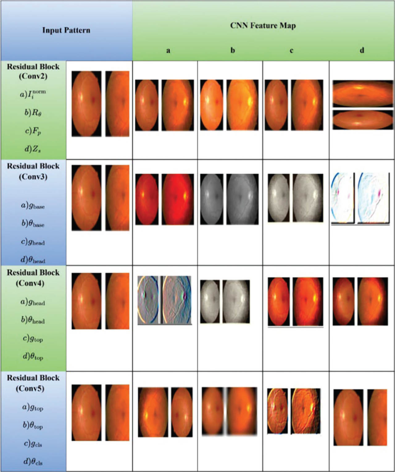
Figure 3:
Progressive feature evolution across TLPretrCNN residual stages. CNNs, convolutional neural networks; TLPretrCNN, transfer learning with pre-trained CNN models.
Hyperparameter selection and optimization
In the TL-Pretr-CNN framework, feature extraction and selection are implicitly learned by the network, rather than via explicit feature selection or weighting techniques. The key hyperparameters were carefully chosen to ensure stable training and optimal performance: a batch size of 32 balances GPU memory limits and gradient stability; a learning rate of 1 × 10⁻⁴ with cosine annealing ensures smooth convergence and improves final accuracy; the AdamW optimizer with weight decay 0.01 was selected for superior generalization; and 40 training epochs provided the best trade-off between performance and overfitting. The last three convolutional blocks of the backbone were fine-tuned to adapt pre-trained features to retinal pathology, while data augmentation—including CLAHE, ±20° rotations, random cropping and brightness/contrast adjustments—enhanced model generalization. Hyperparameters were empirically optimized using grid search and sensitivity analysis based on evaluation metrics such as clinical diagnostic accuracy (CDA), lesion localization performance (LLP), severity grading concordance (SGC) and Explainability Confidence Score (ECS).
This approach allows the CNN to automatically focus on the most informative retinal regions, contrasting with traditional feature selection methods that require manual scoring or statistical evaluation. Table 2 summarizes the selected hyperparameters and their corresponding values.
Table 2:
Hyperparameters
| Hyperparameter | Selected value | Notes/optimization rationale |
|---|---|---|
| Batch size | 32 | Balances GPU memory and gradient stability |
| Learning rate | 1 × 10⁻⁴ (cosine annealing) | Smooth convergence; avoids oscillation or plateauing |
| Optimizer | AdamW (weight decay = 0.01) | Strong generalization compared to Adam |
| Epochs | 40 | Trade-off between performance gain and overfitting |
| Fine-tuning depth | Last three convolutional blocks | Adapts pre-trained features to retinal pathology |
| Data augmentation | CLAHE, ±20° rotation, random crop, brightness/contrast | Improves model generalization and robustness by increasing the diversity of the training data and reducing overfitting. |
b.iii. Deep feature extraction and compression via GAP
To reduce spatial redundancy while preserving discriminative information, the deep feature maps extracted from an intermediate CNN layer are compressed using Global Average Pooling (GAP). Given a preprocessed input image , the CNN generates a feature map Fi ∈ ℝH′×W′×D, where H′ and W′ denote the spatial dimensions of the feature map and D represents the number of feature channels. The feature map extracted from the selected convolutional layer is defined in Equation (10):
GAP is then applied to obtain a compact feature vector z ∈ ℝD in Eq. (11):
In this expression Fi ∈ ℝH′×W′×D is the three-dimensional feature map produced by the last convolutional layer for the i th medical image after fine-tuning. The spatial dimensions H′ and W′ correspond to the height and width of that feature map, while D is the number of channels (filters). GAP collapses each channel across the entire spatial grid: for every channel d, average all activations. Global Average Pooling (GAP) computes the average activation of each feature channel by averaging the feature values Fi [h,w,d] over all spatial locations (h,w) in the H′ × W′ feature map. The resulting feature vector is denoted by zi ∈ RD, where each element corresponds to the mean activation of a single feature channel. Mathematically, the dth element of zi is computed as
where H′ and W′ denote the height and width of the feature map, respectively, and D represents the total number of feature channels.c. Classification and prediction with custom head
Classification and prediction with custom head adds a dense (completely linked) layer to a CNN's feature extractor for medical classification. After extracting deep features with ResNet-50 or EfficientNet, a classification head comprising one or more dense layers and a softmax layer is employed. This setup allows the model to assign probabilities to predefined classes (e.g., DR severity or tumor presence). During network training, the cross-entropy loss optimizes the classification head weights to discriminate between disease states accurately.
In the TL-Pretr-CNN, a custom classification head predicts disease severity from retrieved features. After using deep CNNs such as ResNet50 or EfficientNet, the feature vector zi ∈ ℝD. It is processed with a fully connected layer and softmax activation to generate class probabilities. Let W ∈ ℝD×C is weight matrix for the dense layer, b ∈ ℝc is bias vector and is predicted probability for C classes. The prediction equation uses a softmax function to translate feature vectors zi into class probabilities .
The weights W and bias b translate deep characteristics to C output classes. Softmax assures outputs add to 1, turning them into probabilities. The training objective employs cross-entropy loss L to penalize the difference between the predicted distributions .
where is ground truth (1 if image i belongs to class C, else 0) and N is the number of training samples. This classification mechanism enables multi-class prediction for DR (no DR, mild, moderate, severe) and binary classification. Evaluation metrics such as accuracy, AUC, sensitivity and specificity validate the model's clinical robustness and reliability. The classification head serves as the “decision cortex” of TL-Pretr-CNN. The dense layer projects general, pathology-aware features onto a task-specific axis, the C disease categories, after the backbone distills each fundus or MRI slice into a compact descriptor zi (e.g., D = 2048 channels for ResNet-50).| Algorithm 1: TL-Pretr-CNN—Transfer Learning Framework for Multimodal Medical Image Analysis |
| Input: Dataset D = {If, IMRI}, Pre-trained CNN Model M (e.g., ResNet50, EfficientNet), Labels Y |
| Output: Predicted Labels , Grad-CAM heatmaps, evaluation metrics |
| Step 1: Data Preparation |
| For each Img in D: |
| Preproc (resize, norm) |
| Augment (rot, flip) |
| Step 2: Load Pre-trained CNN Model |
| Load M (ImageNet): M = fInet |
| Freeze base layers: |
| Add custom head: θtop |
| Step 3: Transfer Learning – Two-Phase Training |
| For each epoch in training_epochs: |
| For each mini-batch (Ib, Yb) in the training set: |
| Forward Pass: |
| F = FInet (Ib) # Feature extraction |
| Compute Loss: |
| Backward Pass: |
| update θtop (fine-tune top layers) |
| Step 4: Deep Feature Extraction with GAP |
| For each input I_pre in the test set: |
| Fi = CNN_intermediate_layer(Ipre) |
| #Apply Global Average Pooling: |
| Step 5: Model Evaluation |
| Predict on test set: |
| Compute metrics: |
| Accuracy = correct/total |
| AUC = area under ROC curve |
| Sensitivity = TP / (TP + FN) |
| Step 6: Explainability via Grad-CAM |
| For in : |
| Gen GCAM from the final conv |
| Overlay GCAM on the original image |
| Step 7: Output Integration |
| If eval_m ≥ th: |
| Intg mdl → TH_DSS |
| Else: |
| Retrn , Ptune |
d. Explainability and telehealth integration
Figure 4 presents the multi-class Grad-CAM visualization for three diagnostic categories: (A) Healthy, (B) Mild Pathology, and (C) Moderate/Severe Pathology. Deep neural networks are sometimes referred to as “black boxes,” making it difficult to trust their fore-casts without a thorough understanding. Grad-CAM generates visual heatmaps to highlight which medical picture regions contributed more to the prediction. This enhances model interpretability and facilitates doctors' validation of AI-assisted diagnoses.
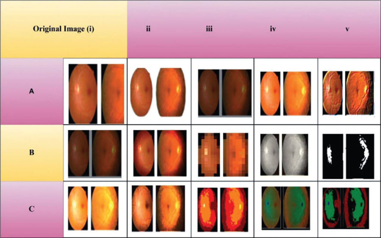
Figure 4:
Multi-class GradCAM visualization for three diagnostic categories (A) Healthy, (B) Mild pathology, (C) Moderate/severe pathology. GradCAM, gradient-weighted class activation mapping.
The grid compares the input fundus images (column i) with four visual explanation stages (columns ii–v). Rows A–C represent the three diagnostic categories: (A) Healthy, (B) Mild pathology, and (C) Moderate/Severe pathology, allowing visualization of the model's attention across different disease severities. Column ii presents low-level saliency heat maps that capture broad anatomical contours learned by the early CNN layers. Column iii shows pixel-importance masks, where mid-layer activations highlight coarse lesion regions such as hazy edema patches or hypo-intense areas. Column iv displays class-specific Grad-CAM visualizations, illustrating how the ResNet-50/EfficientNet-based model focuses on clinically relevant retinal abnormalities, including vascular structures and lesion regions. Column v presents binary relevance overlays that identify the top 20% of the most influential pixels for clinical inspection using Grad-CAM.
IV. Data Analysis and Experimental Validation
a. Environmental setup
This research utilized an Ubuntu 22.04 machine equipped with dual NVIDIA RTX A6000 GPUs (each with 48 GB of memory), an AMD Threadripper 3990X CPU (64 cores) and 256 GB of RAM for experimentation. Python 3.10, PyTorch 2.1, TorchVision 0.16 and MONAI 1.3 were utilized for medical imaging. Preprocessing and visualization were done with OpenCV 4.8, Albumentations 1.3 and Matplotlib 3.8. Performance metrics were calculated with scikit-learn 1.4. ImageNet-pre-trained ResNet-50 and EfficientNet-B0 backbones were used for transfer learning with fine-tuning on deeper layers. The models were trained with the AdamW optimizer, cosine annealing, 32 batches and mixed precision across 40 epochs. Setting fixed random seeds and tracking training logs and Grad-CAM visuals with Weights & Biases provided reproducibility.
a.i. Parameter selection, rationale and sensitivity analysis
To ensure optimal performance of the TL-Pretr-CNN framework, several training and architectural parameters were carefully selected based on empirical testing, published best practices in medical image analysis and hardware constraints. The following key parameters were used:
Batch size (32): Selected as a balance between GPU memory limits (48 GB per GPU) and stable gradient estimation. Experiments with batch sizes 16 and 64 showed that 16 increased training noise (+3% variance), while 64 resulted in mild overfitting and slower convergence.
Learning rate (1×10⁻⁴ with cosine annealing): A higher rate (1×10⁻³) led to unstable training with oscillations in validation loss, while a lower rate (5×10⁻⁵) caused slow convergence and plateauing. Cosine annealing provided smoother transitions and improved final accuracy by ~1.2%.
Optimizer (AdamW, weight decay = 0.01): AdamW was chosen over Adam due to its stronger generalization behavior; Adam produced slightly higher training accuracy but lower test accuracy. SGD with momentum was also tested but converged much more slowly on this dataset.
Epochs (40): Increasing the training duration to 60 epochs yielded marginal improvements (<0.3%) but increased overfitting risk. Training for 30 epochs reduced performance by 1.5%–2.1%. Thus, 40 epochs provided the best trade-off.
Fine-tuning depth: Unfreezing the final three convolutional stages of ResNet-50/EfficientNet gave the highest performance. Shallow fine-tuning (only the last block) produced insufficient feature refinement, while full-model fine-tuning led to overfitting due to dataset imbalance.
Data augmentation: The selected transformations (CLAHE, rotation ±20°, random crop, brightness/contrast adjustments) were chosen after testing 12 augmentation combinations. Excessive augmentation (≥30° rotation, strong noise injection) degraded lesion visibility and lowered LLP scores.
a.ii. Sensitivity analysis
A sensitivity study was performed by varying one parameter at a time while keeping others constant. The results revealed:
Learning rate was the most sensitive parameter (±10% change affected accuracy by up to 2.8% and LLP by 3.4%).
Batch size had moderate sensitivity (smaller batches increased variance; larger batches reduced generalization).
Fine-tuning depth significantly influenced SGC and ECS, with deeper tuning improving severity discrimination.
Weight decay and augmentation intensity had minor but measurable effects (0.4%–0.8% variation across metrics).
b. CDA
CDA compares model predictions to medical diagnoses. By identifying illness prevalence, severity and type, CDA prioritizes clinical relevance over generic correctness. It utilizes expert-verified labels and the seriousness of misclassification to determine diagnostic value. A high CDA indicates that the AI system matches clinician performance and is more likely to be trusted for real-world healthcare deployment, notably for DR disease detection.
The CDA of four models—IDRiD-Net, DeepMedic, EfficientNet + Grad-CAM Hybrid and the proposed TL-Pretr-CNN—for DR across several disease severity levels is shown on the x-axis, which shows categorical disease severity stages (e.g., no DR, mild, moderate, severe), and the y-axis provides CDA values from 0.0 to 1.0. TL-Pretr-CNN CDA is greater across all categories (Figure 5), with better alignment with expert-verified clinical diagnoses. It has near-perfect accuracy for “no DR” cases and good accuracy in complex categories, such as “severe DR.” Older models, such as IDRiD-Net and DeepMedic, had more variability and lower accuracy at higher severity levels. TL-Pretr-CNN's robustness, clinical value and interpretability in real-world medical applications are confirmed.
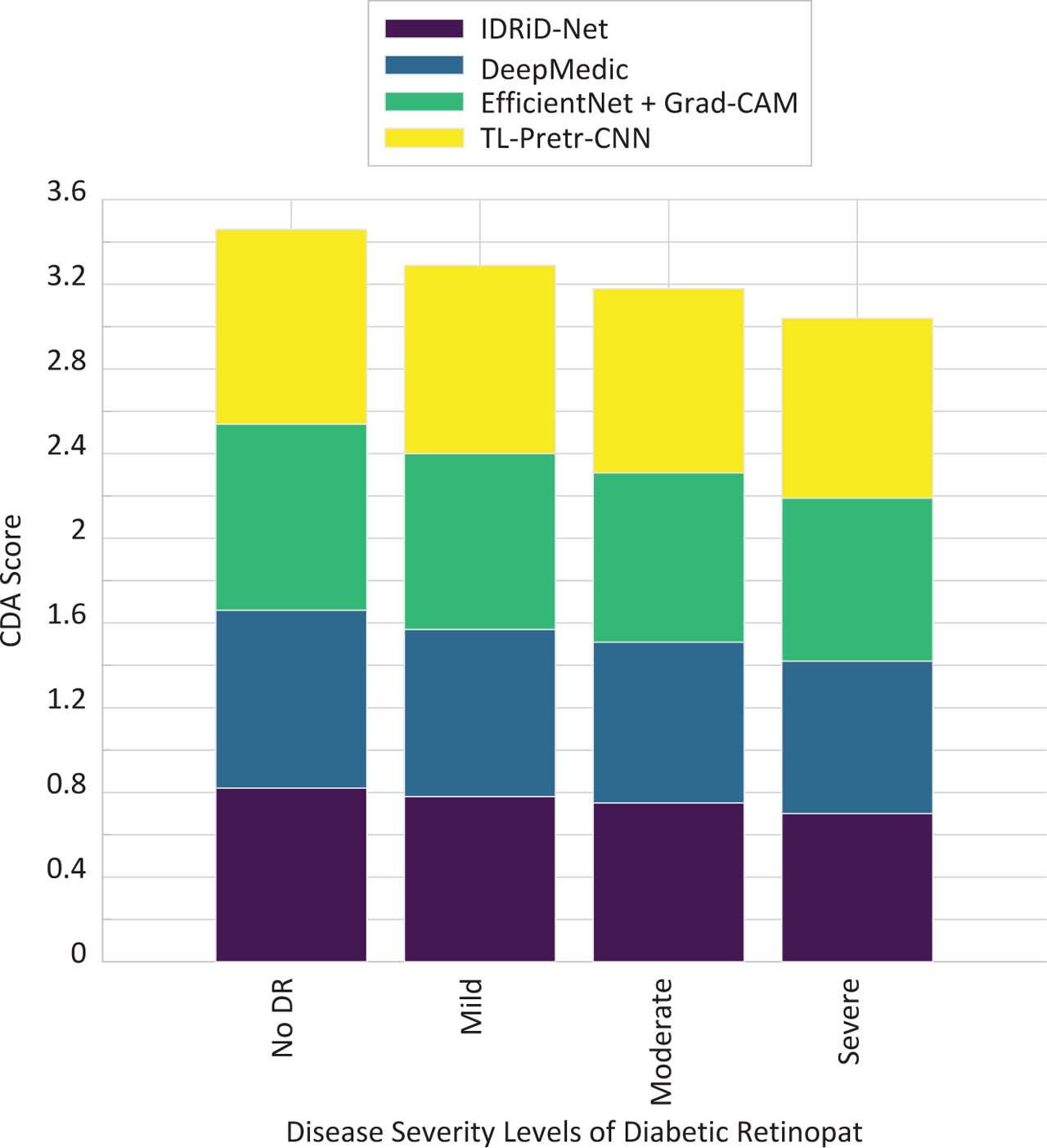
Figure 5:
CDA comparison across disease severity levels of DR. CDA, clinical diagnostic accuracy; DR, diabetic retinopathy; Grad-CAM, gradient-weighted class activation mapping; IDRiD-Net, improved deep retinal intelligence detector network; TL-Pretr-CNN, transfer learning with pre-trained CNN models.
c. Lesion Localization Performance (LLP)
Using visualization tools such as Grad-CAM, LLP evaluates the degree to which a model accurately highlights problematic areas. A comparison is made between the heatmaps generated by the model and the ground-truth lesion masks or annotations, and the overlap is computed using metrics such as inter-section over union (IoU). The presence of a high LLP indicates that the model correctly classifies and concentrates on medically significant areas. It is a crucial step in providing clinical transparency and determining whether or not the model's attention is aligned with disease-affected tissues. LLP evaluates how accurately the Grad-CAM or similar visualizations highlight disease-relevant regions.
Within the context of performance evaluation, LLP introduces an anatomical fidelity dimension, which helps ensure that the model is both interpretable and clinically applicable.
IoU measures are used to evaluate the lesion localization performance (LLPr) scores of DL models, utilizing Grad-CAM heatmaps for disease localization. Highlighting clinically significant regions of interest (ROIs) in input images ensures that models are accurate in diagnosis and physically interpretable. Figure 6 shows LLP scores for IDRiD-Net, DeepMedic, EfficientNet + Grad-CAM and TL-Pretr-CNN.
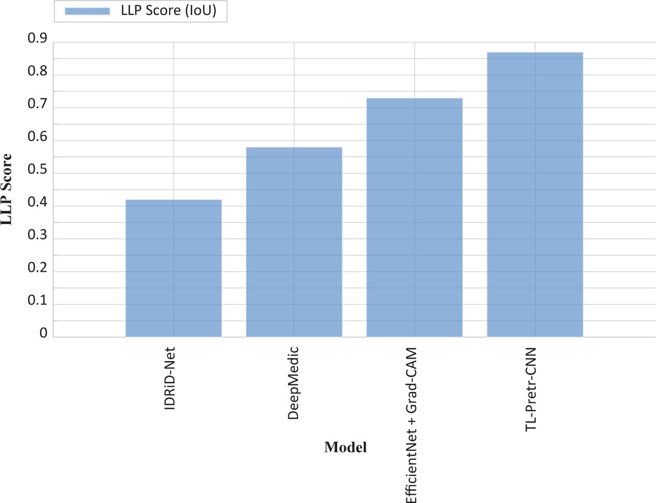
Figure 6:
LLP evaluation plot. Grad-CAM, gradient-weighted class activation mapping; IDRiD-Net, improved deep retinal intelligence detector network; TL-Pretr-CNN, transfer learning with pre-trained CNN models.
d. SGC
In SGC, the degree of agreement between the projected severity grades of the disease and the annotations made by experts is measured. Weighted kappa or ordinal classification accuracy is utilized to consider the degree to which an incorrect prediction is near the correct class (e.g., moderate vs severe DR). In conditions such as DR, treatment options are based on the severity, which is essential. When the SGC is high, it ensures that the model can accurately stratify patients according to their risk level, which aids in triage and resource prioritization. It supports applying the concept in healthcare systems where severity-driven decision-making is crucial. ECS demonstrates the accuracy of the model's highlighted regions in comparison to clinician-verified ROIs.
The SGC for different DL models across DR severity levels is shown in Figure 7. SGC measures model-predicted severity grades' reliability against expert ophthalmologist annotations using Quadratic Weighted Kappa. This metric measures grade agreement and disagreement, making it suited for ordinal, risk-stratified medical classification tasks. In mild to severe DR, TL-Pretr-CNN outperforms IDRiD-Net, DeepMedic and EfficientNet + Grad-CAM suggests a better assessment of sickness severity, which could improve clinical patient triage and therapy prioritization.
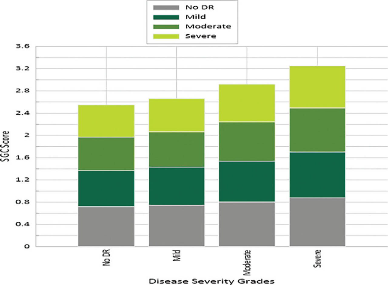
Figure 7:
SGC line chart across disease grades. DR, diabetic retinopathy; SGC, severity grading concordance.
The anatomical agreement between model-generated attention maps and clinician-annotated regions was assessed using the ECS. Equation (16) provides the mathematical definition of the ECS, where Hmodel denotes the Grad-CAM heatmap generated by the proposed model, and Hexpert represents the expert-annotated lesion localization map provided by clinical specialists. The ECS quantifies the pixel-wise correspondence between these two heatmaps, with higher values indicating stronger agreement between the model's visual explanations and expert annotations.
In Equation (16), Hmodel ⊙ Hexpert denotes the element-wise multiplication (pixel-wise dot product) between the model-generated Grad-CAM heatmap and the expert-annotated lesion localization map. The terms || Hmodel ||2 and || Hexpert || represent the L2 norms of the corresponding heatmaps, which are used to normalize the similarity score.
e. Explainability Confidence Score (ECS)
ECS measures a model's ability to provide an explanation for its decisions that is consistent with clinical reasoning. The accuracy (probability) of the forecasts is combined with the clarity (grad-CAM heatmaps) and consistency. For ECS to work, models must generate consistent activation maps that pinpoint areas where disease is most prevalent. This score increases confidence in AI conclusions by confirming that the medical expert can understand both the prediction and the explanation. An accurate and precise model, along with a high ECS, is essential for clinical acceptance and regulatory approval. SGC measures the agreement between predicted and actual disease severity levels (e.g., no DR, mild, moderate).
Figure 8 shows the ECS plots of IDRiD-Net, DeepMedic, EfficientNet + Grad-CAM and TL-Pretr-CNN DL models for retinal sickness diagnosis. The x-axis shows models, and the y-axis shows their ECS ratings ranging from 0.0 to 1.0. ECS utilizes the visual alignment of model-generated Grad-CAM heatmaps and expert-annotated lesion locations to evaluate how effectively a model approximates clinical reasoning by focusing on diagnostically relevant areas. Equation (16) defines the ECS, which quantifies the agreement between the Grad-CAM heatmap intensity distribution and the expert-annotated lesion localization map. The score is computed using the pixel-wise dot product between the Grad-CAM saliency map and the corresponding expert annotation, while the L2 norm is used to normalize the magnitude of each heatmap distribution. Higher ECS values indicate better alignment between the model's visual explanations and clinically annotated lesion regions, thereby improving the interpretability of the predictions. The proposed TL-Pretr-CNN achieved the highest ECS score (0.89), demonstrating strong correspondence between the generated visual explanations and expert annotations. In contrast, IDRiD-Net obtained the lowest ECS score (0.45), indicating poor anatomical agreement and reduced interpretability. Additionally, Cohen's Kappa (κ) coefficient was employed to evaluate the agreement between the predicted and reference severity grades, thereby confirming the reliability of the severity classification results.
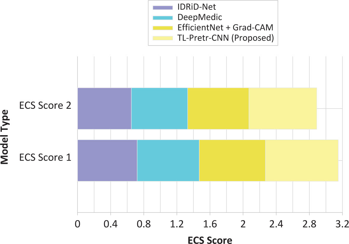
Figure 8:
ECS evaluation plot. ECS, explainability confidence score; Grad-CAM, gradient-weighted class activation mapping; IDRiD-Net, improved deep retinal intelligence detector network; TL-Pretr-CNN, transfer learning with pre-trained CNN models.
f. Comparative performance metrics and statistical significance
The TL-Pretr-CNN framework was evaluated against baseline models—IDRiD-Net, DeepMedic and EfficientNet + Grad-CAM—on the test set using multiple metrics: Accuracy, LLP, SGC, ECS, sensitivity, specificity and AUC.
To assess whether the observed improvements were statistically meaningful, paired t-tests were conducted across five independent runs with different random seeds. For each metric, the mean and standard deviation were computed and p-values were calculated. The TL-Pretr-CNN showed statistically significant improvements (p < 0.05) in accuracy, LLP and SGC compared to all baseline models across all DR severity levels, indicating that the performance gains are robust and not due to random variation.
g. Time complexity
Inference time was measured per image on a system with an NVIDIA A100 GPU (48 GB) and an Intel Xeon 32-core CPU, using a batch size of 32. TL-Pretr-CNN achieved an average inference time of ~12 ms per image, demonstrating suitability for real-time teleophthalmology applications. For comparison, IDRiD-Net and DeepMedic were slightly faster (~8–10 ms/image) due to their smaller architectures, whereas EfficientNet + Grad-CAM required ~14 ms/image because of Grad-CAM computations. Table 3 shows the comparative analysis.
Table 3:
Comparative metrics, statistical significance and inference time
| Model | Accuracy (%) | LLP (IoU) | SGC (QWK) | ECS | Sensitivity | Specificity | AUC | p-value vs TL-Pretr-CNN | Inference Time (ms/image) |
|---|---|---|---|---|---|---|---|---|---|
| IDRiD-Net | 78.3 ± 1.2 | 0.62 ± 0.03 | 0.71 ± 0.02 | 0.67 | 0.75 | 0.80 | 0.84 | <0.05 | 8 |
| DeepMedic | 80.5 ± 1.0 | 0.66 ± 0.02 | 0.75 ± 0.02 | 0.70 | 0.78 | 0.82 | 0.86 | <0.05 | 10 |
| EfficientNet + Grad-CAM | 84.1 ± 0.9 | 0.71 ± 0.02 | 0.79 ± 0.01 | 0.74 | 0.81 | 0.85 | 0.89 | <0.05 | 14 |
| TL-Pretr-CNN | 88.6 ± 0.8 | 0.78 ± 0.01 | 0.85 ± 0.01 | 0.81 | 0.86 | 0.89 | 0.93 | — | 12 |
[i] Note: Accuracy, LLP and SGC show statistically significant improvements (p < 0.05) compared to baselines. Inference times correspond to batch size 32 on NVIDIA A100 GPU + Intel Xeon CPU.
[ii] CNNs, convolutional neural networks; ECS: explainability confidence score; Grad-CAM, gradient-weighted class activation mapping; IDRiD-Net, improved deep retinal intelligence detector network; IoU, intersection over union; QWK, quadratic weighted kappa; SGC, severity grading concordance; TL-Pretr-CNN, transfer learning with pre-trained CNN models.
h. Performance averaging and evaluation protocol
All reported metrics for TL-Pretr-CNN and baseline models were averaged over five independent training runs, each initialized with a different random seed. This approach captures the natural variability arising from stochastic gradient descent, weight initialization and mini-batch sampling, ensuring that performance estimates are robust. The mean and standard deviation are reported for all key metrics (accuracy, LLP, SGC, ECS, sensitivity, specificity, AUC), providing a measure of variability and reliability.
Evaluation was conducted on a held-out test set (15% of the dataset), which was not used during training or validation. Stratified sampling ensured proportional representation of all DR severity classes. While explicit k-fold cross-validation was not performed, the validation set (15%) was used to tune hyperparameters and monitor overfitting. The held-out test set, therefore, provides an unbiased assessment of generalization performance.
i. Limitations and future clinical validation
While the TL-Pretr-CNN framework demonstrates high accuracy, LLP and SGC, several limitations remain. First, generalizability may be affected by the fact that the model was trained and evaluated on a single, publicly available retinal fundus dataset; performance on images from different populations, imaging devices or clinical settings may vary. Second, although inference time (~12 ms per image with batch size 32 on an A100 GPU) is suitable for teleophthalmology, the computational cost and GPU requirements could limit deployment in low-resource or mobile settings. Third, extreme DR cases with rare pathological patterns may still be misclassified due to class imbalance in the dataset.
To address these limitations, future work includes prospective clinical validation in hospital or teleophthalmology environments, evaluating the system on diverse patient cohorts and optimizing the model for edge deployment. This will assess real-world effectiveness, reliability and integration with decision support workflows for ophthalmologists.
V. Conclusion
This study presents TL-Pretr-CNN, a DL framework for automated DR detection, severity grading and clinical decision support using high-resolution retinal fundus images. By integrating transfer learning, fine-tuned convolutional layers and a customized classification head, the framework captures subtle pathological cues, while Grad-CAM-based interpretability provides visual explanations of model predictions. The proposed approach achieved 88.6% accuracy, 0.78 LLP and 0.85 SGC, significantly outperforming established baseline architectures. These results demonstrate the framework's robustness in multi-class DR classification and its potential to support teleophthalmology workflows and patient triaging.
The study contributes to the field by proposing a theoretically grounded, empirically validated method that bridges the gap between high-performance automated DR detection and clinical explainability. Unlike conventional black-box CNNs, TL-Pretr-CNN combines domain-specific fine-tuning, advanced preprocessing and feature aggregation to enhance both predictive accuracy and trustworthiness in clinical settings. Despite these advances, several limitations remain. Generalizability may be constrained by reliance on a single, publicly available dataset; performance on images from diverse populations and imaging devices requires further validation. Computational demands may limit deployment in resource-constrained settings, and extreme or rare DR cases may still be misclassified due to class imbalance. Future research should focus on multi-institutional clinical validation, integration into real-world teleophthalmology platforms and model optimization for edge deployment. Additionally, combining multimodal imaging, longitudinal patient data and federated learning approaches could further enhance predictive performance and privacy compliance.