
I. Introduction
The myocardial infarction (MI), also known as a heart attack, is one of the most serious forms of coronary heart disease and occurs as a result of sudden decreased blood flow to the myocardium. This decrease is commonly due to the rupture of atherosclerotic plaque and then the formation of thrombus in one of the coronary arteries, which causes myocardial ischemia and incurable tissue damage unless it is timely repercussed. Diagnosis of MI clinically is based mainly on electrocardiographic (ECG) defects and biochemical methods of cardiac biomarkers, most notably cardiac troponin I and cardiac troponin T, which are extremely sensitive in detecting myocardial injury [1]. These diagnostic tools are effective, but by their nature, they are reactive, meaning that they only confirm the existence of myocardial damage after it has happened. In addition to its acute physiological effects, MI has a significant long-term and long-lasting effect on the quality of life of patients, which leads to disability, frequent hospitalization and death. On a systemic level, it is astonishing that the increasing number of MIs puts significant pressure on healthcare systems, especially in low- and middle-income areas. This is particularly high in Asia, where the region carries over 60% of the world's cardiovascular disease burden due to a booming population, urbanization, aging population and relocation to a sedentary lifestyle [2].
Cardiovascular risk is natural, multifactorial and lifelong. Epidemiological data have shown that clustering of modifiable and non-modifiable factors, such as high blood pressure, diabetes mellitus, obesity, dyslipidemia, physical inactivity, smoking and psychosocial stress, gradually worsens the health of the cardiovascular system, especially in the elderly [3]. Weakness, cryostasis, inadvertent weight loss, decreased physical activity and slow gait have become crucial intermediaries of negative cardiovascular disease. Longitudinal designs of initially disease-free populations have demonstrated that frailty status is a big factor that increases the risk of further cardiovascular events, including MI [4]. Simultaneously, genetic and biochemical biomarkers, including lipoprotein (a), have been of interest in their causal role in atherosclerosis and residual cardiovascular risk, thereby making the stratification of risk even more difficult [5].
Electrical and structural heart defects often enhance age-related cardiovascular vulnerability. The European Heart Rhythm Association has provided clinical consensus statements that indicate that frail and elderly patients are disproportionately affected by arrhythmias and, therefore, require different management approaches [6]. Recent breakthroughs in signal processing and deep learning (DL) have made it possible to detect arrhythmia automatically based on ECG data, and DL architectures such as DenseNet can perform heartbeat classification tasks very well [6]. Nevertheless, even with single-lead ECG-based devices, enhancing the signal quality, the oversight of clinicians is still needed, and automated interpretations might not be enough to make a definite clinical decision-making, especially related to atrial fibrillation management [7]. The growth of wearables and Internet of Medical Things technology has expanded cardiovascular monitoring to nonclinical environments. Signal sensors of photoplethysmography on consumer-level wearables and smartphones have been effectively interpreted using window-based algorithms to measure the heart rhythm [8], and the internet of things (IoT)-based ECG sensor modules have been used to monitor heart rate in real time [9]. These methods are scalable and can provide ongoing data capture but are in many cases restricted to short-term physiological measurements as opposed to long-term MI risk prediction. Additionally, determinants of lifestyle and behavior are often not properly represented or implicitly modeled in such systems.
Simultaneously, DL and machine learning (ML) methods have been actively used to predict cardiovascular diseases based on structured clinical data. Research with features derived from ECG signals (skewness, kurtosis, entropy and fractal dimension) has shown promising results in classification [10, 11], and benchmark datasets, including the Massachusetts Institute of Technology–Beth Israel Hospital Arrhythmia Database (MIT-BIH) Arrhythmia Database, have been commonly used to test DL models in arrhythmia detection [12, 13]. Other studies have also used conventional datasets, such as the Cleveland and Statlog repositories, to train ML models, such as random forest (RF), Support Vector Machines (SVMs), Logistic Regression, K-Nearest Neighbors and Naive Bayes (NB), and evaluate the performance with accuracy, precision, recall, F1 score and Area Under the Curve (AUC) metrics [14,15,16]. Though it is claimed to have high accuracy, these datasets are comparatively small, feature-constrained and often artificially balanced, which make them less applicable in the real world.
Recent studies have examined enhancement and ensemble methods as a way of improving predictive performance to deal with data imbalance. Bidirectional Long Short-Term Memory (LSTM) models trained as autoencoders have been suggested in the prediction of heart diseases, and they have been shown to be highly accurate on several datasets [17]. Other methods of parameter optimization, such as the GridSearch CV, have also been used to enhance the performance of the model on large-scale data [18, 19]. To solve class imbalance and missing data, generative methods such as generative adversarial network (GAN)-based augmentation, Attribute GANs and modified versions of the synthetic minority oversampling technique (SMOTE) [20, 21] have been proposed, and they are shown to improve recall and AUC of minority groups [22]. However, such techniques usually bring synthetic artifacts and model complexity and can impair interpretability. In spite of these developments, a number of key constraints are still present. Most current methods primarily focus on general accuracy rather than sensitivity to minority classes, use a great deal of signal-level or in-clinic data, or do not incorporate physiological measurements, comorbidities and lifestyle behaviors [22] into a single predictive model. This means that there is a potential to permit high-risk people to go unnoticed, delay the use of preventive interventions, result in avoidable instances of acute events and increase healthcare expenditures. Such weaknesses also contribute to worsening health inequities, in that conventional models fall short in characterizing lifestyle- and socioeconomic-based risk profiles. In order to fill this gap, the current study suggests a large-scale, interpretable and imbalance-aware MI risk prediction framework that incorporates physiological signals, comorbid diseases to disorder and lifestyle variables. It represents MI risk prediction as an anomaly detection problem as a reflection of the real-world prevalence patterns and exponential linear unit (ELU) [23], RF model to improve the sensitivity of the minority class. Extensive comparative analyses are made against current models of ML and DL [24, 25], and Shapley additive explanations (SHAP)-based [26] interpretability is utilized to ensure clinical transparency and reliability.
These restrictions have no abstract effects. Unattended at-risk cases lead to the loss of preventive care and preventable acute and high healthcare expenditures. They indirectly strengthen health inequities by population disadvantages whose risk profiles are more determined by lifestyle and socioeconomic factors than by overt clinical pathology. There is still a knowledge gap, then: the discipline has not yet developed a predictive framework on a large-scale, interpretable, imbalance-aware predictive framework that makes meaningful use of physiological, comorbidity and lifestyle data. This is one of the gaps that will be addressed in the current study. The objective of the study is to construct and test a large-scale MI risk prediction model to include physiological, comorbidities and lifestyle variables. Specifically, it seeks to:
(i) formulate MI risk as an anomaly detection problem reflecting real-world class imbalance;
(ii) apply a SMOTE model for balancing the clinical dataset
(iii) propose an ELU on the RF model to enhance minority-class sensitivity;
(iv) conduct a comprehensive comparative evaluation against established ML and DL models; and
(v) interpret model predictions using SHAP and Local Interpretable Model-Agnostic Explanations (LIME) to ensure clinical transparency.
This research article is structured as follows: The dataset, model design, training and evaluation processes are all covered in Section II. The prediction model for determining MI risk based on clinical, physiological and lifestyle factors is the main topic of Section III. The results and analysis, together with accuracy comparisons with current approaches, are presented in Section IV. The study is finally concluded in Section V.
II. Methodology
The quality and diversity of the data are one of the major factors determining the success of ML and DL models, specifically in healthcare settings such as the prediction of the risk of a MI [27]. However, there are technical, clinical and ethical challenges that lie on the way of the process of collecting and systematizing a diverse, balanced and ethically adequate dataset.
a) Inadequate Representation of Some Subpopulations: Urban healthcare data can also be biased in its representation of a particular demographic (e.g., middle-aged urban male) and ignore the rural population or older people. This leads to biased models that do not even work well when used in diverse settings.
b) Ethnic and Socioeconomic Inequities: MI is manifested in different ethnic groups and genders under the effects of hereditary, lifestyle and environmental factors. A nondiverse dataset can ignore important patterns or associations, which makes such projections unreliable in response to an underrepresented population. The dataset used in this study was developed based on patient-level records, which record diverse demographic, physiological, clinical and lifestyle factors related to MI risk. Some demographical characteristics are age, gender and patient identification number. Physiological variables such as body mass index (BMI), systolic and diastolic blood pressure, heart rate, respiration rate, blood sugar level and stress level are examples of physiological variables. Also, comorbidities (diabetes, heart disease and sleep apnea) and life-style issues (smoking, physical activity and diet) were carefully noted down. The choice of these traits has been to give a comprehensive image of cardiovascular health to allow the identification of both usual clinical risk factors and the determination of both behavioral and psychological influences on the MI risk. As can be seen in Table 1, this dataset indicates that there is a vast range in individual patients in terms of age, comorbidity and lifestyle preferences. The age of the patients was between 23 and 89, and the demographic pattern of the patients was composed of both young adults and older citizens [28]. To guarantee that there was variation in the risk factors with gender, males and females were studied. In a physiological examination, diabetic patients were suggestive of diabetes.
c) The systolic blood pressure was within the range of 111–138 mmHg, and in some cases, it pointed to either hypertension or pre-hypertension. The patients have normal and obese body composition, and therefore, body composition influences cardiovascular stress. Heart disease, sleep apnea and stress problems have been observed in people as one of the known risk factors of comorbidities assessment. The lifestyle factors take into consideration multiple patients who had a high risk of behaviors, including smoking, sedentary lifestyle and junk foods.
Table 1:
Sample dataset of patients' MI risk study.
| PID | Gender | Age (years) | Stress level | Blood sugar | Resp. rate (breaths/min) | Heart rate (bpm) | Blood pressure (SBP/DBP) | BMI status | Comorbidities | Lifestyle factors |
|---|---|---|---|---|---|---|---|---|---|---|
| 2 | M | 77 | High | Elevated | 22 | 63 | 126/84 | Normal | Heart disease, diabetes | Non-smoker, healthy diet |
| 7 | M | 43 | High | Normal | 20 | 81 | 118/84 | Obese | Heart disease, insomnia | Smoker, junk food |
| 9 | M | 50 | Medium | Normal | 18 | 83 | 111/84 | Normal | None | Smoker, junk food |
| 17 | M | 23 | Medium | Normal | 19 | 83 | 113/86 | Normal | Sleep apnea | Healthy food, active |
| 21 | M | 55 | Low | Normal | 20 | 85 | 126/85 | Normal | None | Non-smoker, active |
| 1 | F | 37 | High | Elevated | 23 | 60 | 124/86 | Over weight | Stress disorder | Smoker, junk food |
| 4 | F | 41 | High | Normal | 22 | 99 | 118/72 | Obese | Sleep apnea | Sedentary, junk food |
| 5 | F | 25 | Medium | Normal | 21 | 69 | 138/76 | Obese | Sleep apnea | Smoker, junk food |
| 8 | F | 72 | Low | Normal | 18 | 96 | 135/77 | Normal | None | Healthy food, active |
| 15 | F | 89 | Low | Normal | 17 | 98 | 127/87 | Normal | None | Non-smoker, balanced |
On the whole, the study highlights the complexity of risk factors of MI, where lifestyle habits and more traditional clinical warning signs (including diabetes and hypertension) combine in another way to determine individual predisposition. Importantly, the risk individualities of patients with unhealthy lifestyle factors (and minor comorbidities) in the younger age group were higher, which supports the prognostic importance of integrating behavior and clinical features in patients.
III. Data Processing and Feature Selection
A comprehensive picture of cardiovascular health can be obtained from the patient's physiological assessment, comorbidities and lifestyle, which affect MI risk in addition to the detection of traditional clinical risk markers. The dataset for this study was constructed using patient-level records that detail a range of demographic, physiological, clinical and lifestyle factors linked to MI risk. Let the input feature vector be represented by X = [x1, x2, x3 ……… xn], where each xi stands for a patient attribute such as age, blood pressure, BMI, blood sugar, heart rate, comorbidities or lifestyle choices. Learning the function f: X→Y is the aim. The chance of MI incidence is shown by Y∈{0,1} (0 = low risk, 1 = high risk).
In order to contextualize patient risk profiles, physiological reference ranges were taken into consideration. The average systolic/diastolic blood pressure readings differ by age and sex: in the 18–39 age group, women usually have 110/68 mmHg and men 119/70 mmHg; in the 40–59 age group, the values rise to 122/74 mmHg for women and 124/77 mmHg for men; and in the 60+ age group, the averages are 139/68 mmHg for women and 133/69 mmHg for men. Adults of any sex typically have a resting heart rate of 60–100 bpm, while their normal respiratory rate is between 12 bpm and 20 bpm. Both sexes were classified according to the same BMI, with 18.5–24.9 kg/m2 being considered normal, 25.0–29.9 kg/m2 being considered overweight and ≥30 kg/m2 being classified as obese. These reference standards offer a point of comparison for the risk of MI [29, 30] in specific patients.
a. Data collection
We gathered 281,934 patient records, making sure each entry was linked to a unique Patient ID for clarity and tracking. At the hospital, trained staff collected clinical details such as blood pressure, heart rate, body temperature, respiratory rate, oxygen saturation and documented physical characteristics, including age, gender, height and weight. All these values were recorded during routine visits and included the exact timestamp. Laboratory results for blood sugar, cholesterol levels, triglycerides, urea and creatinine ratio were added to complete the health profile. To truly understand each person's lifestyle and overall well-being, we invited patients to share details about their diet, smoking habits, daily activities (including exercise and step count) and sleep quality using structured surveys and thoughtful interviews. They also described stress levels, general health and any history of heart disease, diabetes or sleep disorders. Having both objective clinical measurements and honest survey responses gave our dataset a rich, human dimension—ready for meaningful insights into health trends.
b. Data cleaning
Before analysis, a thorough data cleaning procedure was carried out to guarantee the validity and reliability of the data. Biometric, lifestyle and clinical history variables from structured clinical records made up the raw dataset. Cleaning was essential for enhancing data quality and reducing bias because health-care data is sensitive and diverse. A combination of statistical imputation methods and domain-informed decision rules was used to address missing data points. Vital sign missing values, for instance, were imputed using the mean or median within clinically relevant subgroups, while inconsistent or non-recoverable records were not included. Interquartile range thresholds and clinical reference ranges were used to identify outliers, such as physiologically improbable blood pressure or heart rate readings. To avoid duplication bias, duplicate entries, located using distinct patient identifiers, were also eliminated. To guarantee uniformity across all numerical features, units of measurement were standardized. After completing these steps, the final cleaned dataset included 34 columns and 281,934 observations, providing a solid basis for further analysis.
c. Data wrangling
To get the cleaned dataset ready for statistical analysis and ML modeling, data wrangling was done. This involved combining and converting semi-structured and structured variables into a consistent. To get the cleaned dataset ready for statistical analysis and ML modeling, data wrangling was done. format that could be processed computationally.
The SVM model has been implemented only for the reduction of overfitting and abstained from training for MI risk detection due to its long execution time. Anomaly detection has been using SVM to create a new binary target variable called “Anomaly_ SVM” after 19–20 min of execution. This is necessary because the data was fused, and it had both numeric and non-numeric values, for instance, a numeric feature—blood pressure, and a non-numeric—sleep disorder. Because cardiovascular risk is unbalanced in the general population, this unsupervised learning method was selected: 0 for “Normal” patterns, which show no immediate risk of MI, and 1 for “Anomalies” (possible markers of MI risk).
To boost the model operation and interpretability, we distinctly employed the clean cardiovascular dataset consisting of 281,934 patient records with 35 features. A synthetic binary target was generated due to the nonappearance of the pre-defined target label in this dataset based on heart rate deviations. This results in the class distribution of Class 0 (Normal), which consists of 267,824 records, and Class 1 (Anomaly), which consists of 14,110 records. Hence, SMOTE [31, 32, 35, 36] was applied, which produced the result of a balanced training set of 306,186 sample records and a test set of 92,657 sample records. Categorical variables were encoded to expand the feature set to 399 attributes to bring more transparency in the analysis. One-class SVM was used specifically for unsupervised anomaly detection, not for classification. The key reasons were to learn from a normal class, only using highly imbalanced medical data without a proper target column, making it difficult to predict the risk. The traditional SVM used had its own limitations, requiring both classes (Class 0, Class 1) with a ratio of 19:1, which fails with severe imbalance, creating confusion between the normal and the anomaly (Table 2). As the medical features have non-linear relationships, SVM maps data to a higher-dimensional space where categorization is easier. In preventive medicine, we know what normal or healthy looks like, and anomaly detection brought more practicality than supervised classification for rare events. But SVM might result in false warnings before clear disease symptomatic reactions. SMOTE was chosen because it addressed the root cause of imbalance, was model-friendly and compatible with any classifier, preserving information, unlike SVM violating the documents when used numerous times, and enabling transparency, reliability with SHAP and LIME (Figure 1A and B). SMOTE was used after the split to avoid any leakage. SMOTE treated the minority class with equal significance, unlike SVM, which overlooked the same. SMOTE saves the long training time of SVM, creating a balanced training set for reliable model building to identify further potential risk patterns. Although SVM has the ability to learn the risk patterns by providing continuous risk scores, not just binary, SMOTE stepped back in this case. As the dataset is highly unaligned, SVM learnt from normal patterns only, whereas SMOTE had to first solve the imbalance of the dataset. SVM has the power to improve itself according to the recent risk patterns; nonetheless, traditional classifiers failed with data imbalance, enforcing data transformation.
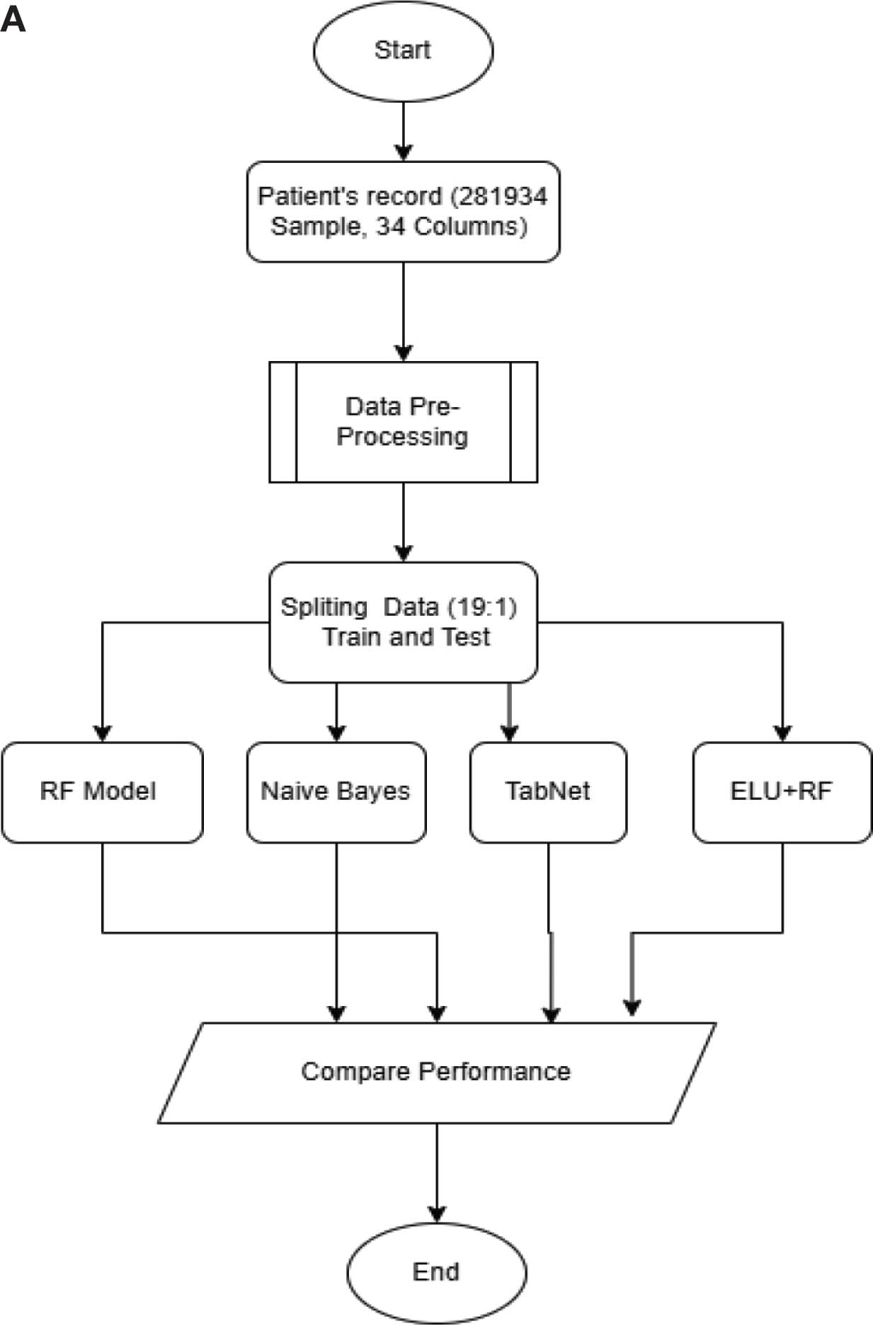
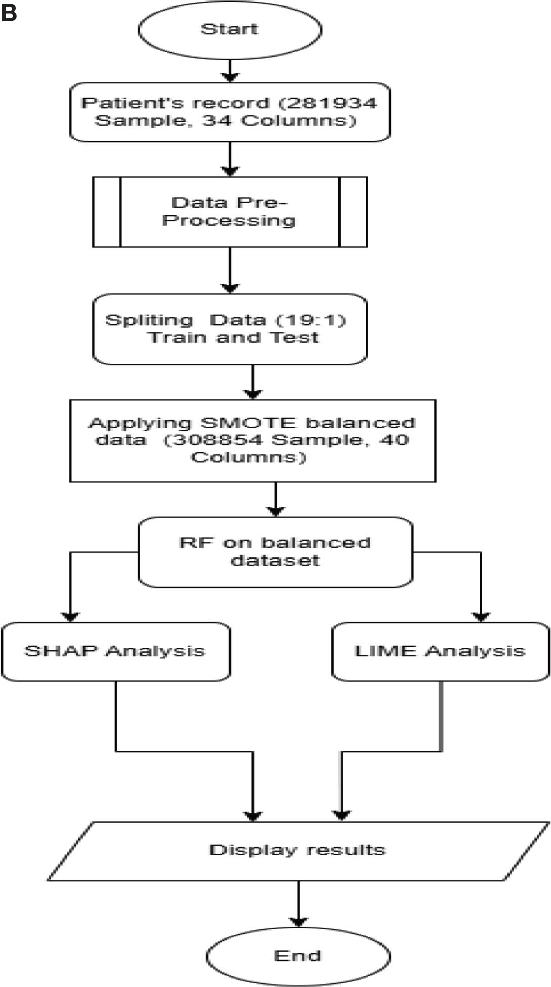
Figure 1:
(A) Evaluation of MI risk with the execution of SVM. (B) MI risk with the execution of SMOTE. ELU, exponential linear unit; MI, myocardial infarction; NB, Naïve Bayes; RF, random forest; SHAP, Shapley additive explanations; SMOTE, synthetic minority oversampling technique; SVM, support vector machine.
Table 2:
Decision boundary comparison.
| Method | Samples properties | Result |
|---|---|---|
| SVM-based: Imbalanced data |
| Boundary optimized for the majority class Anomalies misclassified as normal (high false negatives—dangerous for medical diagnosis) |
| SMOTE-based: Balanced data |
| Boundary fairly separates both classes Better classification of the minority class (Better sensitivity—critical for early detection) |
c.i. Feature extraction by SHAP
SHAP is used in the current study due to its explain-ability-based feature extraction and interpretation system to determine which determinants of MI risk are the most significant [22]. SHAP uses cooperative game theory and assigns a value of contribution to each input feature by allocating the prediction of a model to all the features fairly according to the marginal contribution of the variables. This methodology is especially appropriate to clinical risk modeling, as transparency, consistency and interpretability on an individual level are required.
where F denotes the full set of features, S represents a subset of features excluding, f(·) is the predictive model. This is defined to compute the average marginal contribution of a feature i of all the possible feature coalitions, with local accuracy, consistency and additivity [23]. In this research, SHAP is used with the ELU on the RF model proposed, and the computation of the accurate Shapley values of tree-based ensembles is performed with the aid of the Tree SHAP algorithm. On a global level, the mean absolute SHAP values are summed up over the dataset to bring out the most significant predictors of MI risk, which is, in essence, a form of importance-based feature extraction. This facilitates the induction of clinically significant drivers, such as metabolic indicators, stress-related variables and lifestyle habits that have a consistent increase in predicted MI risk. Locally, SHAP offers patient-specific interpretations by estimating the effect of individual characteristics on the model output by moving the model in the direction of high-risk or low-risk categories. This individual attribution assists in clinical reasoning as it exposes the reason why a given patient is considered anomalous and not just through aggregate statistics [24]. Through the incorporation of SHAP, the current study will guarantee that the MI risk predictions can be accurate, interpretable, clinically transparent and in accordance with the decision-making in the real world.d. Data analysis
To measure the risk distribution as represented in Figure 2 and investigate important distinctions between the normal and anomaly classes, the labeled dataset was examined. Among the 281,934 medical records, about 95% of the records, or 267,824 records, were categorized as normal. An increased risk of MI was indicated by the 14,110 records (approximately 5%) that were categorized as anomalies. This classification confirms the usefulness of anomaly detection in extensive patient screening and represents actual clinical prevalence rates.
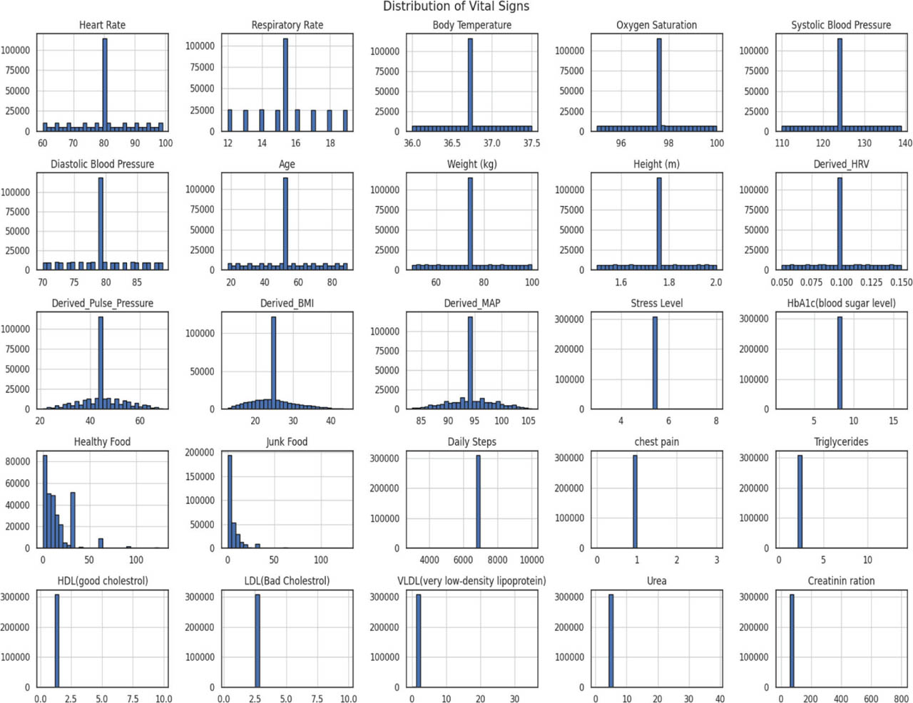
Figure 2:
Distribution plot of patients' vitals. BMI, body mass index; VLDL, very low-density lipoprotein.
The implementation of such models in preventive care settings, where early identification is crucial but rare cases must not be disregarded, is supported by the comparatively low percentage of high-risk cases. Group-wise comparisons of important variables (such as mean blood pressure, stress scores and sleep quality) between the normal and anomaly groups may be part of additional statistical analysis. To find the best predictors of MI risk, multivariate analysis and feature importance rankings are also planned. Both clinical decision-making and the creation of customized risk assessment instruments can benefit from these insights.
Figure 3 interprets the patient's vital parameter correlation heatmap. The heatmap highlights important patterns related to MI risk prediction by demonstrating the degree of correlation and inter-relationships among physiological measures (blood pressure, heart rate, respiratory rate, BMI and blood sugar). The mathematical expressions of different models are presented as follows:
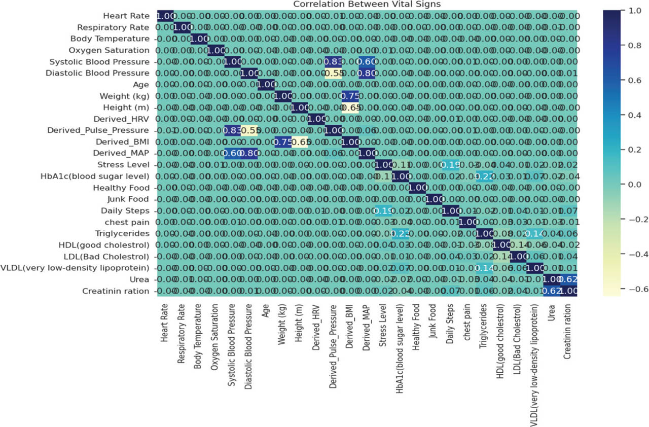
Figure 3:
Correlation heat map for vitals. BMI, body mass index; VLDL, very low-density lipoprotein.
d.i. RF
Here, Yj is the prediction of the jth decision tree, and the final output is obtained by majority voting across n trees.
d.ii. NB
Given a feature vector X = [x1, x2 ……… xn], class variable C and P(C) is the prior probability of class CCC, P(xi/C) is the likelihood of the feature and P(X) is the evidence. The probability of MI risk is expressed in Eq. (2).
d.iii. TabNet [33, 34]
Let a feature vector X = [x1, x2 ……… xn], at each decision step t.
Here, fatt is the attention module, and Ht−1 is the aggregated feature representation from previous steps [25, 26]. The selected features Ft are transformed and aggregated to produce the final output .
d.iv. ELU
The ELU is an activation function used in DL, designed to overcome some limitations of traditional functions such as Rectified Linear Unit (ReLU) [27, 28]. Here, α is a positive constant set to 1, and for an input x:
IV. Result and Analysis
In this investigation, the dataset has been thoroughly cleaned to eliminate missing values and superfluous features, and finally, the dataset consists of 281,934 samples with 34 variables following preprocessing. Anomaly is the main outcome variable, which was created as a binary classifier to represent the state of cardiovascular health: Class 0: 267,824 samples (normal) and 14,110 samples in Class 1 (anomaly—risk of MI). With normal instances making up roughly 80.0% of the dataset and anomalous cases making up only 20.0%, this distribution demonstrates a notable class imbalance. In medical datasets, MI is relatively unusual in comparison to healthy or normal observations, which creates an imbalance. A good prediction model requires a well-balanced dataset. In cases where the dataset is highly unbalanced, the majority of current classification techniques typically perform badly on minority class examples. To create predictive models that work, a dataset must be balanced. Many conventional classification methods perform badly on the minority class in unbalanced scenarios. The test set is randomly stratified to avoid any biases. SVMs, which use kernel methods to handle the fused data (i.e., vital signs and other attributes), were used to identify normal and abnormal situations in order to address this problem. By learning a decision boundary (hyperplane) that distinguishes typical cases from possible outliers, the one-class SVM (OC-SVM) was utilized to detect anomalies. The normal observations were designated as 0 (normal), while the outliers that were found were designated as 1 (anomaly). Using kernel methods, SVMs can handle nonlinear classification and perform well in high-dimensional fields. Because it only learns from the “normal” class and recognizes deviations as anomalies, the OC-SVM is particularly well-suited for anomaly identification. RF is a decision tree-based ensemble approach, resilient to missing values and noise resistant to overfitting brought on by cross-tree averaging and effective in managing categories. Bayes Naïve, a baseline model that is helpful for comparison to more intricate techniques, is fast and capable of managing both textual and categorical data. A DL model called TabNet was created especially for tabular data based on attention to concentrate on the most important aspects of automatic feature selection and end-to-end learning.
Figure 4 represents the confusion matrices of TabNet, RF and NB models to show how well they classify cardiovascular health cases into normal (Class 0) and abnormal (Class 1) categories. RF works well in situations where reducing false positives or false alarms is crucial. Despite having more false positives, Naïve Bayes is better suited when recall or sensitivity to anomalies is the main concern. When there is a risk of both false positives and false negatives, TabNet offers a balanced trade-off and might be the better option. The SHAP model [35, 36] was implemented to show the feature importance on which the decisions of the models depend, as described in Figure 5.
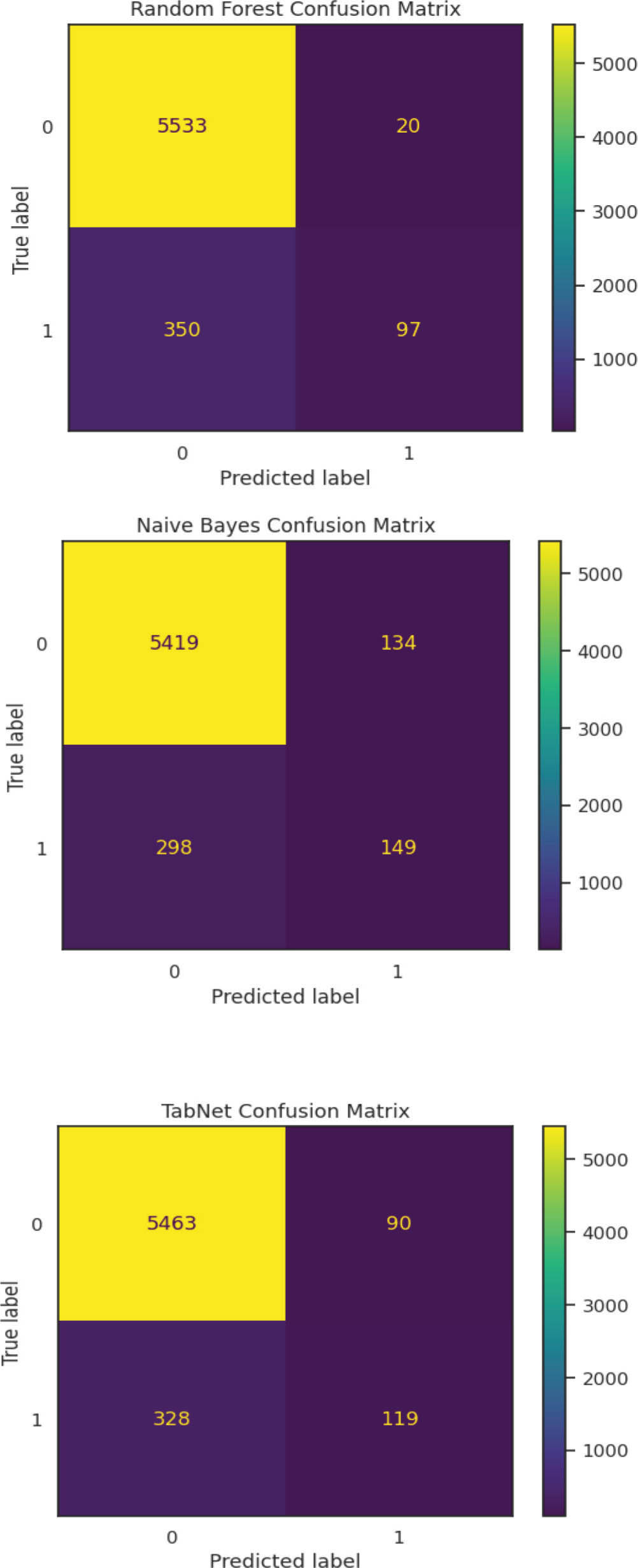
Figure 4:
Confusion matrix for models TabNet, RF, NB. NB, Naïve Bayes; RF, random forest.
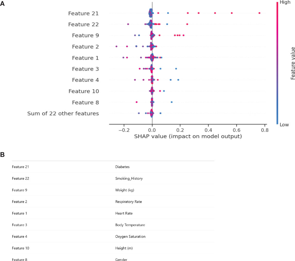
Figure 5:
(A) Feature impact on model output. (B) Feature impact on model output. SHAP, Shapley additive explanations.
With the greatest influence on the categorization outcomes, features 21, 22 and 9 stood out as the most significant factors among all the predictors. While low values (shown in blue) moved predictions closer to the normal class, high values (shown in red) of these traits were linked to positive SHAP contributions, which increased the likelihood of anomaly prediction. While such as Features 4, 10 and 8 showed comparatively less influence, intermediate features such as Features 2, 1 and 3 showed moderate contributions. The remaining features contributed slightly but not insignificantly to the model when combined as the “sum of 22 other features.”
Tables 4–6 display the training results of RF, NB and TabNet, respectively, with their performance parameter. Training RF over anomaly (1), it was concluded that out of all the predicted positives, the normals (0) were 94% and anomalies (1) 82%. Out of actual positives, the 0s that were predicted correctly are 100% and 21% for 1s. Moving on to the F1 score, it denotes that 97% normal cases were detected accurately and 33% anomalies were detected, which is a weak balance. This glimpse of weak balance was also shown in Support, where 5,553 cases were detected for normal and 447 for anomalies. Accuracy is 94%, which is quite satisfactory with a little class imbalance. Macro average and weighted average are dominated by the majority, which suggests that the model is suffering from class imbalance. On the other side, NB's and TabNet's precision accuracy for the 1s is lower than RF 53% and 57%, respectively, hence compromising on the accuracy as well. Class 0 dominance allows all three models to reach excellent accuracy (~93%–94%). The minority class (1) recall is extremely low across all models.
Table 4:
Model performance of RF.
| Precision | Recall | F1 score | Support | |
|---|---|---|---|---|
| 0 | 0.94 | 1.00 | 0.97 | 5,553 |
| 1 | 0.82 | 0.21 | 0.33 | 447 |
| Accuracy | 0.94 | 6,000 | ||
| Macro avg | 0.88 | 0.60 | 0.65 | 6,000 |
| Weighted avg | 0.93 | 0.94 | 0.92 | 6,000 |
Table 5:
Model performance of NB.
| Precision | Recall | F1 score | Support | |
|---|---|---|---|---|
| 0 | 0.95 | 0.98 | 0.96 | 5,553 |
| 1 | 0.53 | 0.33 | 0.41 | 447 |
| Accuracy | 0.93 | 6,000 | ||
| Macro avg | 0.74 | 0.65 | 0.68 | 6,000 |
| Weighted avg | 0.92 | 0.93 | 0.92 | 6,000 |
Table 6:
Model performance of TabNet.
| Precision | Recall | F1 score | Support | |
|---|---|---|---|---|
| 0 | 0.94 | 0.98 | 0.96 | 5,553 |
| 1 | 0.57 | 0.27 | 0.36 | 447 |
| Accuracy | 0.93 | 6,000 | ||
| Macro avg | 0.76 | 0.63 | 0.66 | 6,000 |
| Weighted avg | 0.92 | 0.93 | 0.92 | 6,000 |
NB is somewhat better at catching more positives (higher recall), while RF is better at accuracy (fewer false alarms). The minority class (1) is difficult for your models to detect, whereas the dominant class (0) is easily identified. RF misses the majority of Class 1 but hardly ever mislabels Class 0. Although they still have limited performance, NB and TabNet do somewhat better in identifying some Class 1 cases.
In order to fix this imbalance, RF (ELU on RF) was integrated with the ELU activation function. In contrast to ReLU, which truncates all negative values, ELU introduces a smooth nonlinear transformation by permitting modest negative outputs. This characteristic makes it possible to represent minority class samples more accurately (Table 5). Applying a nonlinear transformation, ELU changes the distribution of features to enhance the separability of features by smoothening noise. This improves the quality of the RF split because the decision tree is able to find features of lower impurity. Combining the strengths of both approaches, the technique made use of RF, which is particularly good at managing feature importance and heterogeneous data. With the greatest AUC value of 0.96 in the baseline evaluation in Figure 6, RF demonstrated a remarkable capacity to distinguish between normal and abnormal instances. TabNet obtained the lowest AUC of 0.89, indicating a poorer separation between the two classes, while NB came in second with an AUC of 0.92, indicating reasonable performance. These findings align with the confusion matrix study, which showed that TabNet provided a fair but ineffective trade-off, RF produced fewer false positives and NB collected more anomalies at the expense of precision.
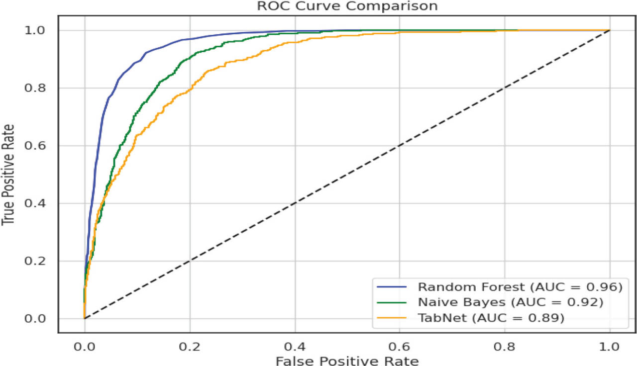
Figure 6:
ROC curve comparison of OC curve comparison of TabNet, and RF. NB, Naïve Bayes; RF, random forest.
Significant progress was noted after the ELU on the RF model (bottom panel) was introduced and displayed in Figure 7A. With an AUC of 0.99, the technique demonstrated almost flawless normal and abnormal class separation. This enhancement shows how well ELU as in Figure 7B generates nonlinear feature transformations that better high-light minority class patterns, which, in turn, improve RF's anomaly detection capabilities as in Table 6. In contrast, TabNet and NB recorded AUCs of 0.95 and 0.93, respectively, whereas standalone RF obtained an AUC of 0.97. The ELU on RF framework showed the greatest effect (Table 7), with the uplift across all models indicating that ELU-driven representations enhanced feature expressiveness.
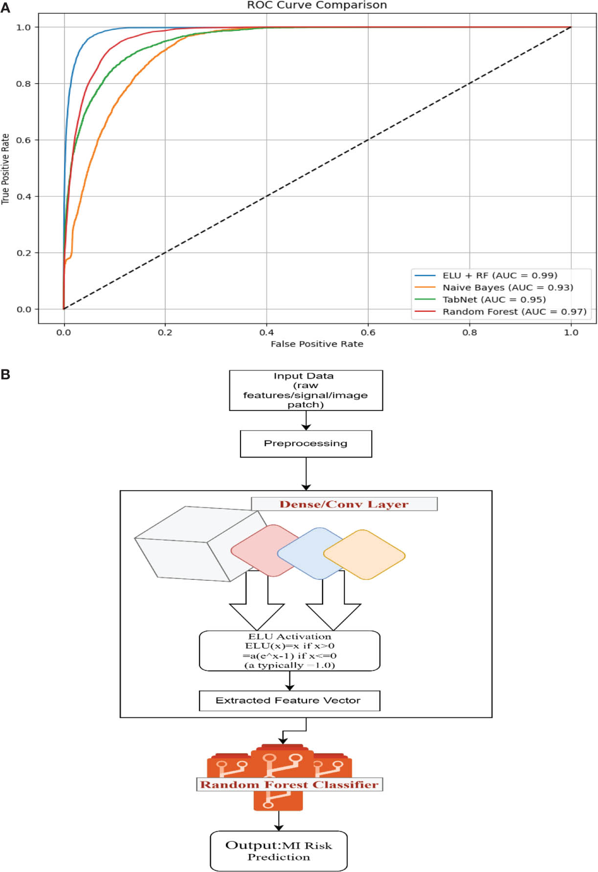
Figure 7:
(A) ROC curve comparison of the enhancing approach. (B) Usage of ELU in the feature extraction layer prior to the RF. ELU, exponential linear unit; MI, myocardial infarction; NB, Naïve Bayes; RF, random forest.
Table 7:
Model performance of ELU on RF.
| Precision | Recall | F1 score | Support | |
|---|---|---|---|---|
| Class 0 | 0.98 | 0.99 | 0.99 | 5,553 |
| Class 1 | 0.90 | 0.85 | 0.88 | 447 |
| Accuracy | - | - | 0.97 | 6,000 |
| Macro avg | 0.94 | 0.92 | 0.93 | 6,000 |
| Weighted avg | 0.97 | 0.97 | 0.97 | 6,000 |
Finally, the Receiver Operating Characteristic (ROC) analysis settles that although Class 0 dominance helps conventional models attain high accuracy, their capacity to identify anomalies is still constrained. The ELU on RF technique is the most successful model for anomaly detection in this study since it not only corrects for this imbalance but also achieves state-of-the-art performance with improved sensitivity and specificity.
a. RF (SMOTE-based)
After the use of SMOTE again the RF Classifier was used on the balanced dataset (Table 8A) and gained an overall accuracy of 99.30%. The classification performance is given in Table 8B.
RF investigated and got hold of the top 15 features in Figure 8, which are important and taken into account for risk prediction; reportedly, Heart Rate is the most important, and Weight is the least. Whereas Derived BMI and Gender Male have been rated second; Respiratory Rate, Oxygen Saturation and Derived_Pulse_Pressure were rated third; Derived Mean Arterial Pressure (MAP) rated fourth; Age is fifth; Systolic Blood Pressure, Derived_Heart Rate Variability (HRV) and Body Temperature stand sixth; Height and Diastolic Blood Pressure stand seventh. The balanced dataset had clearly impacted the importances, unlike the SVM-based RF's irregular mapping.
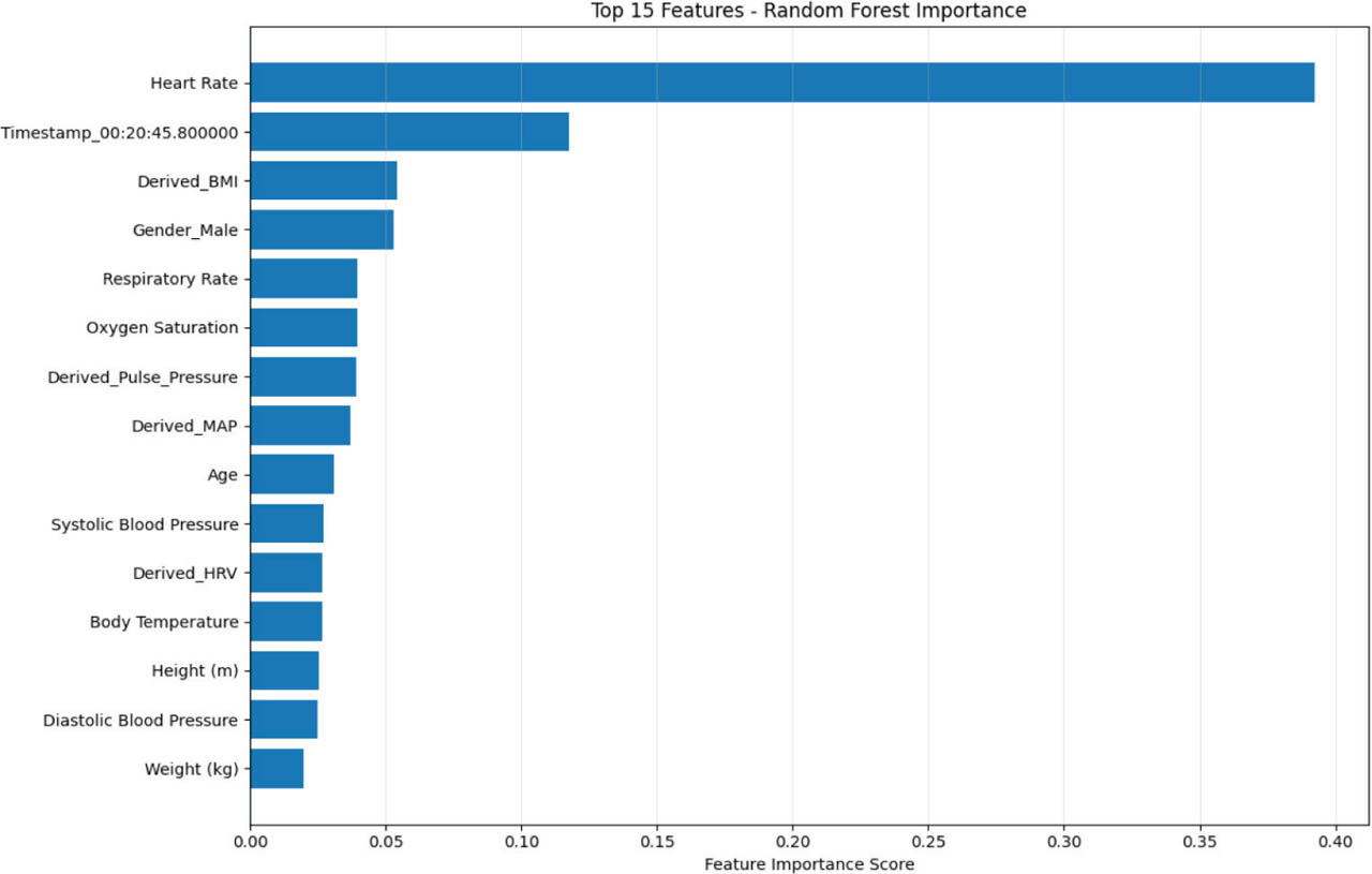
Figure 8:
Investigation of feature importance related to the feature vector. BMI, body mass index; RF, random forest.
Proving that SMOTE had its best use, in Figure 9, RF resulted in true negatives of 64,965, representing patients who were healthy and correctly identified as healthy, preventing patients' unnecessary tests and treatments, and 647 false positives say otherwise. No MI risk was missed; therefore, 0 false negatives. A total of 27,045 patients were detected with MI risk, correctly helping them receive timely medical intervention. As we can observe, an excellent diagnosis of false negatives was the objective behind using SMOTE.
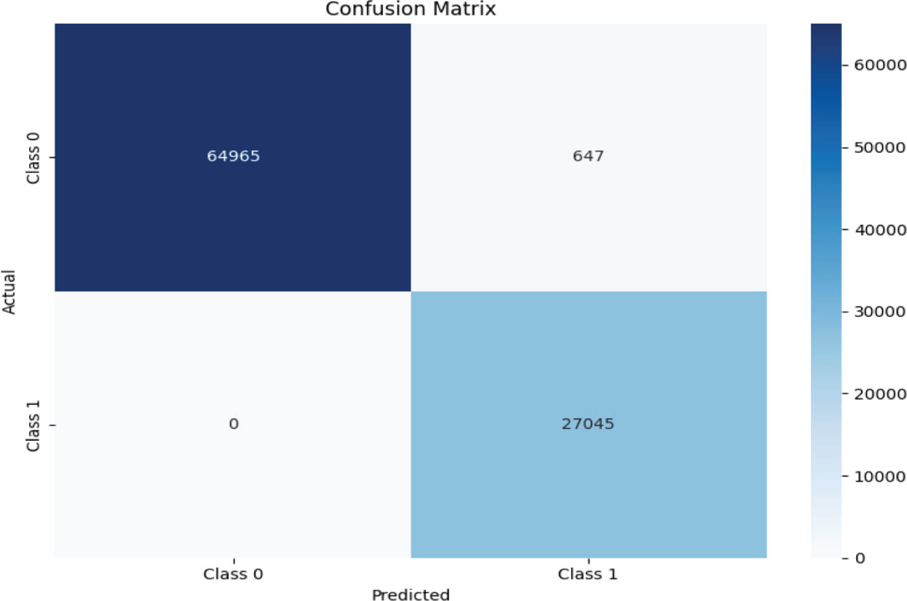
Figure 9:
Confusion matrix of RF following SMOTE. RF, random forest; SMOTE, synthetic minority oversampling technique.
In the SVM-based application, ELU on RF model, where ELU used prior RF for enhancing feature importance as shown in Figure 7B. As RF alone could not deliver a successful value of recall (0.21, missing 79% of high risk) and desired accuracy (94%), mostly due to SVM working on an imbalanced data set overlooking the minority classes and following the normal trend of the dataset. Due to this, it forced us to use an oversampling (SMOTE) model to ensure a balanced dataset with a proper target column “Risk” as well as providing a ratio of 1:1 for the classes. Relying on “Accuracy” (~94%) in an imbalanced dataset is misleading, as it primarily reflects the majority class by ELU on the RF model to prove that the high AUC actually translates to better detection of at-risk patients, not just a better ranking of probabilities. Hence, minority classes were treated equally, and RF delivered a better result. As it has been observed in Figure 11, there has been a massive uplift in the Recall value of 79%, accuracy increased 5.30%, keeping the training time the same, yet enhancing the interpretability of the evaluation. Although in ELU on RF, ELU gave a significant spike in the accuracy and AUC score, as displayed in Figure 10, mainly due to its function in solving imbalance and feature enhancement, and RF decided the final result. Similarly, SMOTE enhanced the features, balancing and providing target column without ignoring minority classes, RF decided the results, but with better accuracy and AUC score.
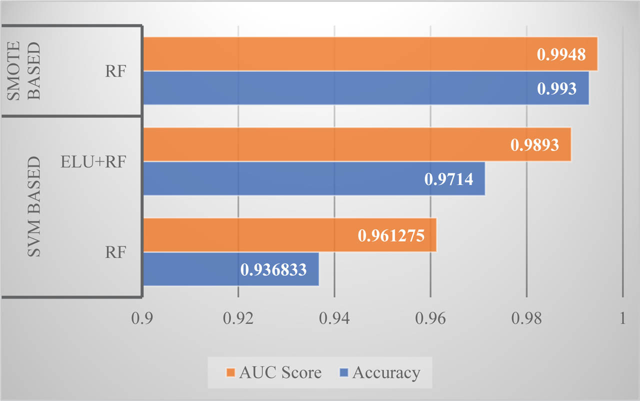
Figure 10:
Comparison of improved accuracy and AUC. ELU, exponential linear unit; RF, random forest; SMOTE, synthetic minority oversampling technique; SVM, support vector machine.
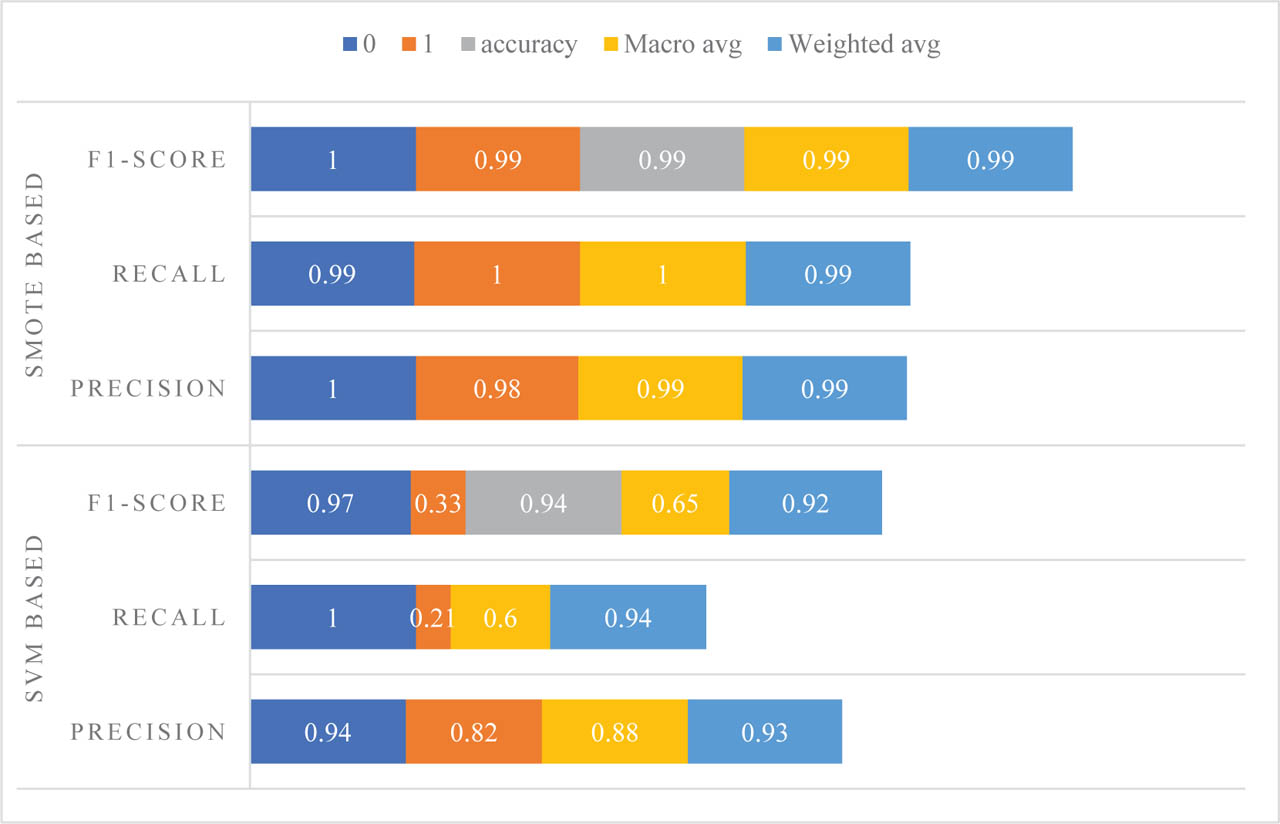
Figure 11:
Metrics comparison of RF. RF, random forest; SMOTE, synthetic minority oversampling technique; SVM, support vector machine.
b. Use of ELU on RF (SMOTE-based)
Later, when ELU on RF was applied under SMOTE, there was not much change in the result from the standard RF and there was no improvement in accuracy (Table 9).
c. Interpretability analysis with SHAP and LIME
To bring better interpretability, we performed comprehensive SHAP and LIME analysis, which provides global and local insights into feature contributions. This method will help clinicians and in understanding the models' decision-making process. SHAP analysis was introduced to quantify the impact of each feature on model predictions. The SHAP summary table disclosed that Heart Rate and Respiratory Rate were the most dominant predictors. Next in line are time-stamped physiological measurements and demographic factors, such as Gender and BMI. Figure 5A and B displays feature importance for “Features 21, 22 and 9,” but these are never mapped back to the 34 input variables, while in Figure 12, mean absolute SHAP values highlighted the top useful features. It can clearly identify the most dominant features, providing them with a distinctive target column, preventing false negatives and also missing out on high-risk trends. Hence, SHAP features deliver the typical clinical decision-making.
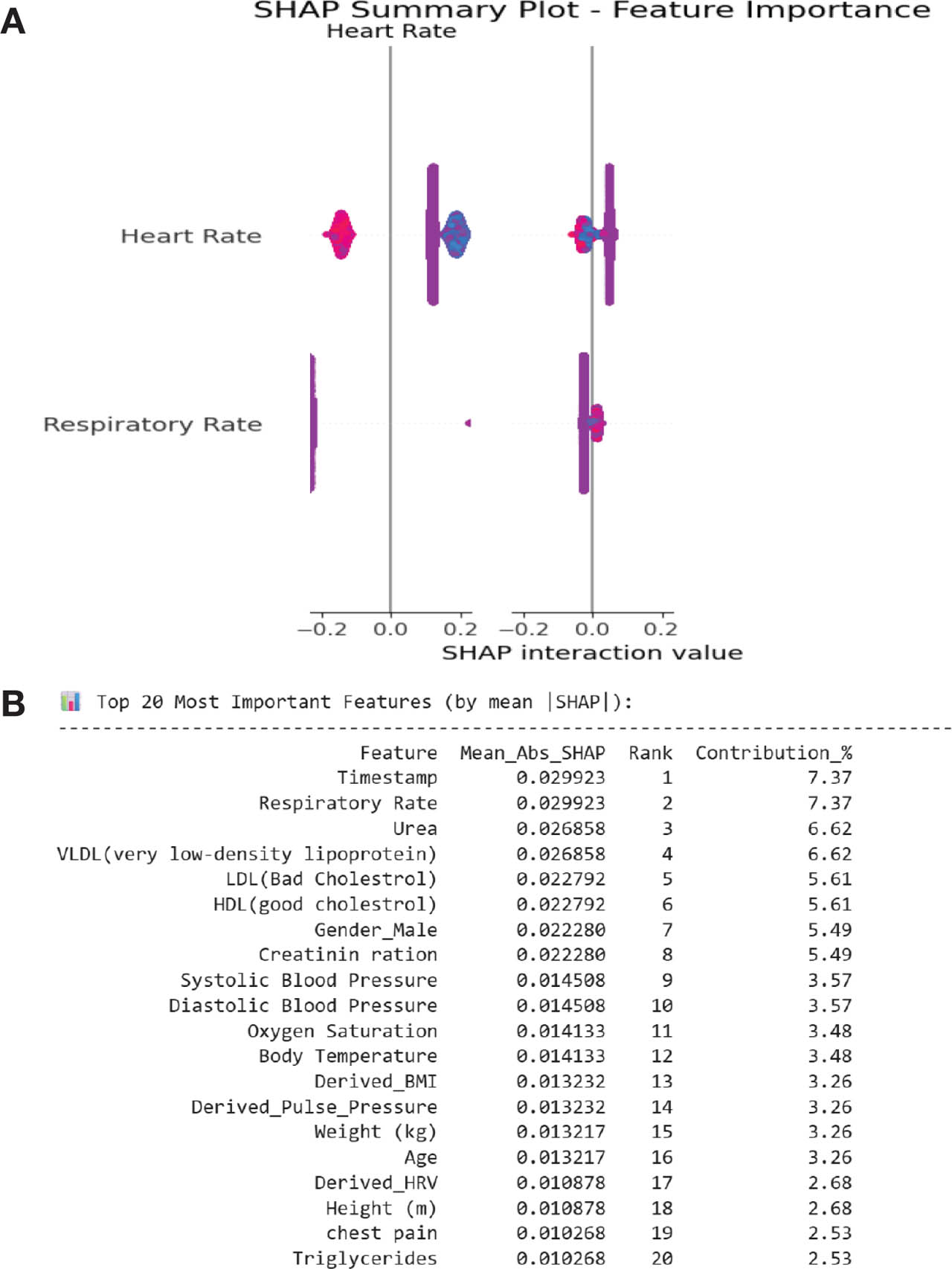
Figure 12:
(A) SHAP for two dominant features. (B) Mean SHAP for features. BMI, body mass index; SHAP, Shapley additive explanations; VLDL, very low-density lipoprotein.
For further segmented analysis, LIME was used to explain the individual predictions, providing insight into how specific patient profiles dominated classification. LIME is used to detect negative and positive values, indicating the direction of each feature's dominance on that prediction for those specific samples after using SMOTE. We have already figured out from Figure 12 that “Heart Rate” has been the most influential feature for most of the attributes. Here, we used a sampling method explanation using LIME, showing the influential features sequentially for each sample. Hence, we have taken three distinctive samples furnished in Table 10.
Table 10:
Samples and their properties.
| Samples | Properties |
|---|---|
| Sample 1 | Sample index: 82,496; true label: 1 (Class 1); predicted probabilities: [0.26460299 0.73539701]; predicted class: 1 (Class 1) |
| Sample 2 | Sample index: 51,516; true label: 0 (Class 0); predicted probabilities: [0.60369369 0.39630631]; predicted class: 0 (Class 0) |
| Sample 3 | Sample index: 55,756; true label: 0 (Class 0); predicted probabilities: [0.624137 0.375863]; predicted class: 0 (Class 0) |
Being the most influential feature, Heart Rate with LIME value of +0.1283 defines the increase of risk for index number 82,496 (Figures 13–15), while Derived Pulse_Pressure is the least influential with LIME value of +0.0032, decreasing risk though leaning to the positive rates indicating chances of high risk. The result was very well expected as the sample index was taken from Class 1 (Risk). Considering sample index 51,516, here we observe that though the Heart Rate is the most dominant feature, it does not include itself in the increasing risk category, whereas the Derived BMI and the Timestamp say otherwise, though not much influential in the reading. The sample index 55,756 has low risk overall, though the timestamp shows a positive value of +0.0023; it does not define risk alone without any other feature in the increasing risk category.
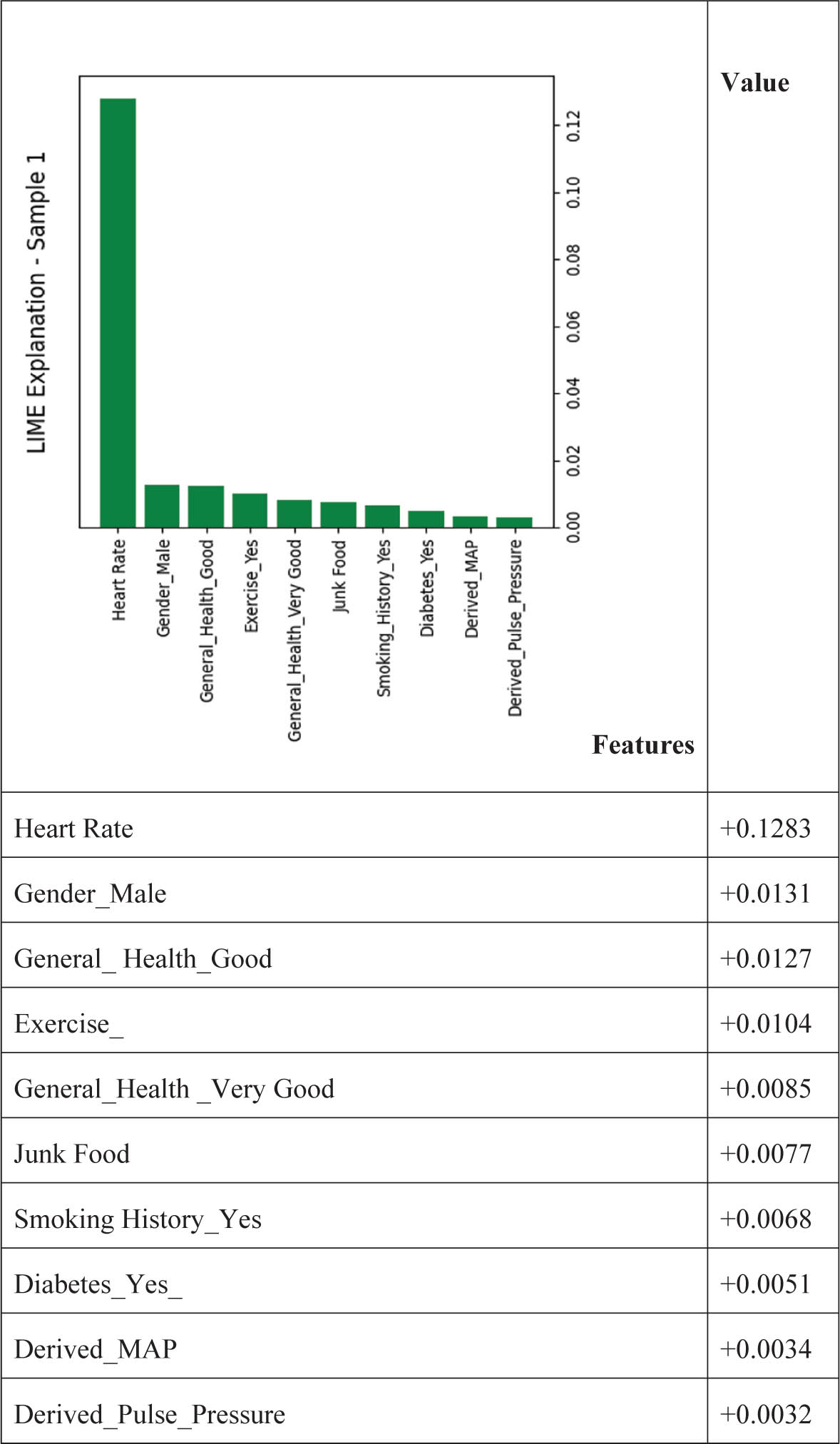
Figure 13:
LIME analysis for sample 1 (Class 1).
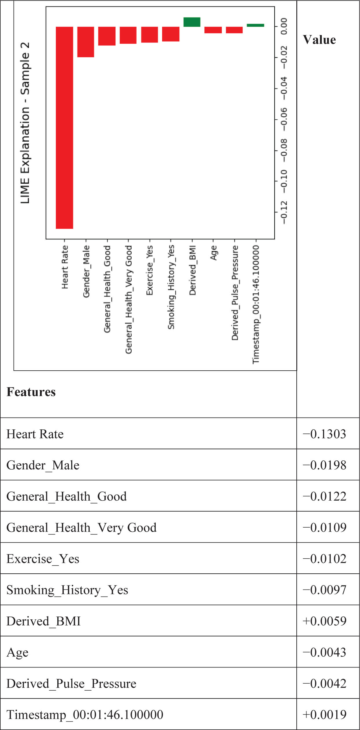
Figure 14:
LIME analysis for sample 2 (Class 0). BMI, body mass index.
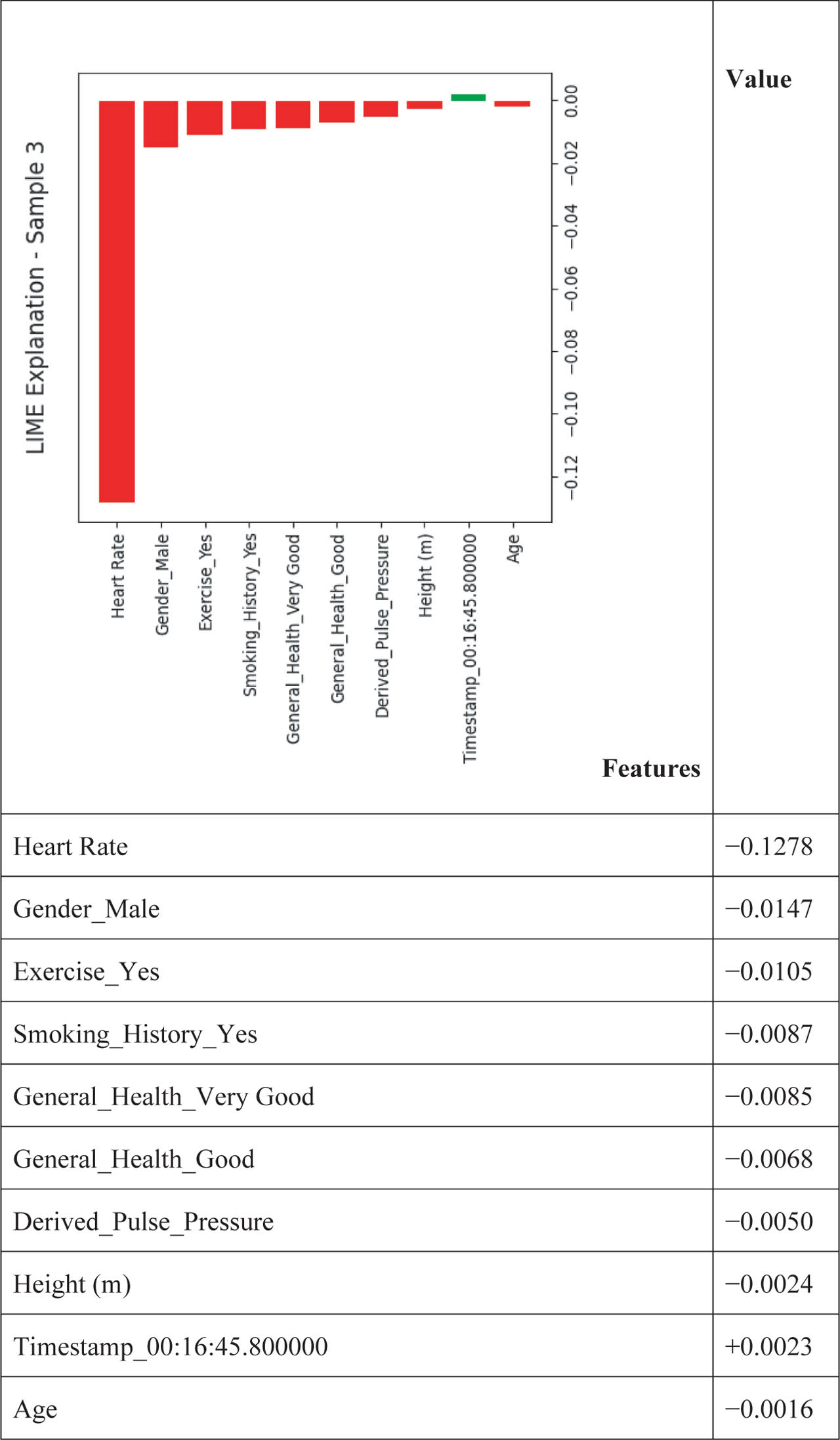
Figure 15:
LIME analysis for sample 3 (Class 0).
V. Conclusion
This paper introduces a scalable and clinically interpretable DL-assisted model for predicting the risk of MI, directly from the physiological, comorbidity and lifestyle data. The traditional ML and DL models were accurate because of the dominance of classes, but they had low detection rates of the minority cases, which are at risk. The frequency of normal cases meant that the old known classifications, such as RF, TabNet and NB, emulated an excellent overall rate; however, they could not detect any anomalies of the minority classes. OC-SVM was applying the right labels to potential high-risk cases, which were examined, identified and analyzed. The ELU and the RF (ELU + RF hybrid) were used to obtain near-perfect classification between normal and high-risk instances (AUC = 0.99), which significantly heightened the sensitivity of the model and represented the minority cases. However, later we found out that the data were heavily imbalanced and had false anomalies and we had to use the oversampling method (SMOTE). SMOTE actually helped in cleaning the dataset and producing a balanced dataset (Class0:Class1–1:1) with better clinical interpretability. Heart rate is the main indicator of cardiovascular stress. Lifestyle and demographic factors (e.g., gender, smoking, diet) significantly regulate risk. Time-series physiological data improve predictivity granularity, supporting real-time monitoring applications. Then, for the risk prediction, we used RF under SMOTE and had an excellent mapped confusion matrix (0 false negatives, 1.00 recall) and accuracy 99.30%, proving that though ELU used to enhance in ELU on RF was a failure due to the imbalanced dataset. Hence, SMOTE-based RF stands out. It is shown that the combination of deep nonlinear representations and ensemble learning can significantly increase anomaly detection in severely imbalanced medical data. This comparative study showed how the type of dataset and the target column are important. The analysis of the importance of features shows that both clinical variables and lifestyle factors are important to predict the risk of MI, which holds importance in interpreting the model. This combined strategy is a general feature that generally high-lights the value of combining lifestyle and comorbidity data with state-of-the-art ML algorithms to improve early MI risk diagnosis, optimize preventative care and provide practical clinical decision-making insights. Extrinsic validation in a wide population and connection to real-time clinical decision support systems will be given attention in the future.
Notes
[8] Ethics Declarations
This study was conducted in accordance with applicable ethical guidelines and regulations. Participation was voluntary, and informed consent was obtained from all participants prior to data collection. Participant confidentiality and privacy were maintained through-out the study, and all collected data were anonymized and stored securely. No procedures were undertaken that could cause harm to participants.
[9] Contributed by Author Contributions
Conceptualization: B. Kundu and T. Sarkar; methodology: T. Sarkar and E Chakraborty; investigation: B. Kundu; formal analysis: T. Sarkar and B. Kundu; software: T. Sarkar and E Chakraborty; writing: T. Sarkar, E Chakraborty and B. Kundu.
[10] Conflicts of interest Conflict of Interest
The authors declare that they have no conflicts of interest.