
I. Introduction
Real data may not exist or cannot be accessible due to some regulations, such as the Digital Personal Data Protection Act, 2023 (India), related to personal information privacy concerns. Also, the existing data may be insufficient or highly imbalanced. So, to overcome the limitations of real-world data, researchers are turning to creating synthetic data, which is rapidly taking over the market. Artificially created data intended to mimic data from the real world is known as synthetic data. It is produced by employing statistical models and algorithms that mimic the relationships, patterns, and traits in actual data. Among other things, synthetic data can be used for reducing bias in data sets, enhancing privacy and security, and training and testing machine learning (ML) algorithms. Non-compliance with the general data protection regulation (GDPR) can result in severe penalties. Businesses that violate the rules risk fines of up to 4% of their yearly worldwide revenue or €20 million, whichever is higher. By addressing privacy and data protection threats highlighted by GDPR compliance rules by the European Union, synthetic data can save you millions of dollars [1]. Synthetic data helps industry overcome obstacles, including a lack of data availability [2], the need for diverse datasets, and data privacy concerns, while also fostering the development of more accurate, equitable, and robust ML models across sectors [3].
Over time, the idea of synthetic data has changed dramatically, moving from basic statistical techniques to sophisticated AI-driven models. To duplicate statistical features without disclosing sensitive information, techniques, such as sampling and resampling, were used to solve data scarcity and privacy concerns [4]. The range of synthetic data has expanded over time due to sophisticated simulation models, such as agent-based modelling, which capture dynamic interactions and behaviors within datasets [5]. Fields, such as epidemiology and the social sciences, were noticeably impacted by these advancements. Synthetic data generation (SDG) advanced substantially when Goodfellow et al. [6] introduced generative adversarial networks (GAN) and variational autoencoders (VAE) [7], which helped to produce more varied and realistic synthetic datasets.
The healthcare sector is beginning to see the benefits of synthetic data, which is increasingly being used to maximize data exchange and, ultimately, as an innovative strategy to the growing need for more privacy [8]. There are many challenges in collecting statistically valid medical data. Many dataset quality issues for AI training can be resolved via generated datasets [9]. While navigating the complex terrain of producing synthetic data, our objective is to extract insights, establish correlations, and offer a comprehensive synopsis of the developing approaches that tackle these complex problems. We seek to identify any potential connection between the requirements for large, balanced datasets, the complexities of managing imbalances, and privacy regulations by carefully examining the reviewed papers. This will help to create a more informed and ethical methodology approach to data-intensive applications in the fields of ML and neural networks. As such, this study provides an overview of ML’s privacy risks as well as privacy-preserving techniques. Then, we explored one privacy preservation method, i.e., SDG techniques, GAN, with emphasis on tabular synthetic data, and evaluation metrics of generated data.
II. Privacy Risks in ML and Privacy Preservation
In ML, privacy risks occur when models unintentionally remember and reveal private information that was utilized for training. Personal information can be extracted from models that appear to be anonymized using methods, such as membership inference attacks and model inversion. This is particularly troubling for industries, such as healthcare and financial services. Secure model deployment, differentiated privacy strategies, and cautious data processing are all necessary for privacy protection. This section first covers possible privacy related attacks in ML and then methods to preserve privacy of data to maintain data privacy.
a. Privacy-related ML attacks
Adversarial knowledge can be used to model the various attack surfaces against ML models [10]. The scope of knowledge ranges from having access to the API of ML to being fully aware of model parameters and the training settings. A variety of scenarios fall somewhere in the middle, such as having little knowledge of training configuration, hyperparameters, and the model’s architecture[10]. In attacks pertaining to privacy, the adversary’s goal is to get access to information that is not supposed to be exposed. Such information can be regarding data, a model, or properties of data.
Membership Inference Attack: Shokri [11] proposed the fundamental attack used to check whether model’s training dataset includes a particular data instance, or not known as membership inference attack. Finding out that a record was used to train a specific model while the adversary is fully aware of it is a sign that information is leaking through the model. In certain situations, it may result in a direct violation of privacy. For instance, it can be determined that a patient has a condition if it is known that the patient’s clinical record was used to train a model linked to that disease [12]. Lastly, the viewpoint of the data owner offers another perspective on these kinds of attacks. In this case, the data owner might be able to examine models to find out if the data access permission has been given or not.
Attribute Inference Attack: Users must answer questions about their age, gender, and other personal details while creating an account to help with user profiling. If hostile third parties manage to steal sensitive user data, the results could be disastrous. However, new studies show that it is highly possible to infer users’ unpublished private information from their interaction history. Age, gender, political affiliation, health, financial position, and other personal details are examples of this type of information. Furthermore, by leveraging the inferred features, the attackers can connect user profiles across platforms and jeopardize anonymity [13]. In such an attribute inference attack [14], the hostile attackers may include advertising, data brokers, or cybercriminals. One example [15] uses the publicly available IMDB user profiles to deanonymize Netflix users successfully.
Property Inference Attacks: The process of deducing dataset attributes that are neither explicitly stored as features nor directly related to the primary learning objective is known as property inference. For instance, extracting data from medical datasets regarding the ratio of boys to girls. An attacker with access to a trained ML model and an attempt to retrieve some in-depth statistics from the training data is the focus of property inference attacks [16]. Any ML model creator is ready to share model prediction, but no other properties like the environment where data is created or part of the data coming from a specific class [17]. Ateniese et al. [18], first invented property inference attack by doing experiments with Hidden Markov Model and Support Vector Machine.
Model Extraction Attack: Attacks using model extraction are thought to be a leading cause of vulnerability in ML. In these attacks, an intruder trains a duplicate model that can replicate the original model’s output by repeatedly querying it [19]. Later, attacks of this nature could be a start to more violent ones, including membership inference [20] or adversarial attacks [21]. In addition to developing surrogate models, a few approaches concentrate on extracting knowledge from the final model, like learning parameters in the objective function [22] or details about different aspects of the neural network architecture, like the activation types, optimization algorithm, and number of layers [23].
b. Privacy-preserving methods to secure privacy
To mitigate the risks and protect privacy, various techniques such as data anonymization and pseudonymization can be employed. In addition to this, some specific methods like differential privacy (DP), local differential privacy (LDP), and privacy-preserving SDG can help us to safeguard sensitive data from inference attacks.
DP: When an adversary tries to infer information about an individual within a dataset, DP can be a solution. It uses mathematical mechanisms, such as Laplace, Gaussian probability distribution, or exponential mechanism, to add random noise in a dataset. It ensures that the adversary cannot identify individual information by comparing the dataset with other datasets. A trade-off between model utility or accuracy and privacy protection is offered by DP. According to the findings of an assessment of ML models that are differentially private against attacks using membership inference, privacy could only be protected if the models’ effectiveness was greatly diminished [24]. If the added noise is reduced, it increases the privacy leakage.
LDP: Traditional DP depends on third-party service providers to create noisy data to maintain privacy and assumes that they are trusted. However, even well-established companies are unable to guarantee their customer’ privacy. For instance, in 2018, leakage of Google + social network users’ data by Google, and 52.5 million user accounts were exposed due to bugs in the Google + API in the same year [25]. This raised questions about trust in the third party to manage user privacy. As a solution, LDP [26] can be used by enabling users to make local changes to their own data on their own computers, with just the modified data being uploaded to the server. Despite its potential, LDP has a limited application scope as data is altered locally independent of other users, and lowers utility as the noise included is very large with an increase in complexity.
Privacy Preserving SDG: Synthetic data refers to artificial data that resembles original data [27]. In case of data scarcity, poor quality data, or improving ML model performance, synthetic data can be used. Along with preserving quality, privacy should be guaranteed when working with sensitive data, such as credit information or medical records. Generation of synthetic data revolves around these two issues. Rather than collection, as it is generated, it does not reveal any private information when privacy constraints are applied. It is important to properly generate synthetic data by adhering to the distribution and patterns of the original data.
III. Privacy Preserving SDG
The statistical properties of synthetic data are identical to those of real data from which it is derived. The only difference is that computer algorithms generate synthetic data while original data are gathered in the real world [27]. Real data’s distribution and correlation between variables are captured by synthetic data. As stated in the study by Nikolenko [28], fake data can be used in ML for three purposes: training ML models, using them for predictions on real data, augmenting data to generate an undersampled part of the data, and maintaining data privacy. According to the literature, numerous techniques have been put out to create synthetic data, each with a specific purpose and use. This study aims to focus on tabular SDG.
a. SDG workflow
Figure 1 represents steps involved in SDG, such as i) data collection, ii) preprocessing, iii) modelling, and iv) evaluation. The very first step is real data collection, ensuring the privacy of sensitive information by following the data regulations and laws. The second step is about data transformation to remove noise and get clean data that is suitable for modelling. This involves identifying and removing missing values, outliers, data normalization, and feature transformation to get good-quality data. The third step involves the generation of synthetic data by maintaining important properties and characteristics of the original data. This includes the development of SDG models, such as statistical models, ML, and deep learning models. The final step is to assess the generated data to check its quality in terms of utility, fidelity, and privacy.

Figure 1:
Workflow of fake data generation.
Figure 2 depicts the increased interest in the study of fake data generation from 2015 to 2025. The figure shows the total number of research publications indexed in the Scopus database annually from 2015 to 2025. It demonstrates a notable rise in the number of publications throughout time.
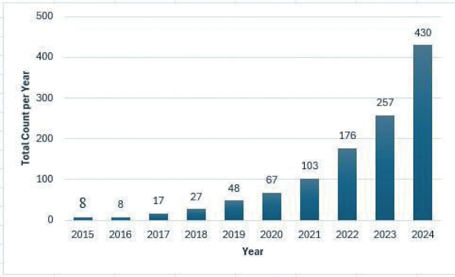
Figure 2:
Total publications per year indexed in the Scopus database from 2015 to 2025.
b. Tabular fake data generation methods
In this part, we attempt to concentrate on previous studies in tabular artificial data generation across sensitive domains, such as healthcare and finance. In addition to tabular SDG, the study covers the metrics for assessing the quality of generated data in terms of utility and fidelity. The study highlights how advanced models, such as GAN, VAE, and large language model, address the challenge of data privacy, data scarcity, and data imbalance.
Programming Rule-Based Approach: To produce data that closely mimics the characteristics and patterns of real-world data, predefined rules, logical constructions, and simulation models are applied during the programmed generation process. These techniques are pretty flexible and can be modified to replicate the same structures, relationships, and patterns found in actual data. The type of programming approach used in practice is a rule-based approach [29]. Establishing rules that reflect the characteristics and connections of the data, putting these rules into code, and running the program to generate synthetic data are the steps involved in rule-based systems. These systems are highly predictable and reproducible because they are deterministic, meaning that the same rules always produce the same outcomes. If links and constraints are clearly specified, this approach is helpful in producing structured data.
Statistical Approach: This method creates synthetic data using statistical or probabilistic techniques based on relationships between variables in actual data and the statistical distribution of data points. Statistical methods based on previous studies include Gaussian copula, Bayesian network, bootstrapping, and multivariate normal distribution (MVND). These methods have been used for the augmentation of data, data transformation, and large-scale data generation. The Gaussian copula method [30] is used to handle missing values in various imputation techniques. It models the dependence on data attributes to build the joint distribution, which can be later used for fake data generation.
IV. SDG Methods
The type and complexity of the data are two of the many variables that affect the choice of a synthetic data production technique. Statistical techniques may be helpful for data that are pretty simple. For more complex datasets, such as structured data like tabular data or unstructured data like photos or videos, deep learning models may be needed.
a. Standard methods
Prior to the emergence of deep learning-based approaches, several conventional techniques were employed for SDG. This section begins with random oversampling (ROS), a simple way to rectify the imbalance of classes by reproducing minority class samples. We then explored the synthetic minority oversampling technique (SMOTE) and its numerous variants, which generate synthetic samples by interpolating existing minority instances. Then, we examined cluster-based oversampling methods, which leverage clustering algorithms to guide the oversampling process by preserving the underlying data distribution. Finally, we analyzed Gaussian mixture models (GMMs), a probabilistic framework that models data distribution as a combination of multiple Gaussian components, enabling the generation of realistic synthetic samples.
ROS: ROS duplicates the minority class instances to add a few observations to the dataset. It does not change the data distribution but instead learns the patterns in data with incorrect distribution. It just replicates the samples rather than generating new ones, so a more advanced method, SMOTE, has been developed. random undersampling (RUS) is a method of removing random instances of majority classes to avoid underrepresentation of minority classes. [31] compared both ROS and RUS and proved that ROS performs better than RUS, as it does not affect the majority class instances by increasing minority class samples.
SMOTE [32]: It is an advanced oversampling method that generates synthetic minority samples rather than simply duplicating existing instances, as done in ROS. The algorithm operates by selecting a minority class sample and identifying the k-nearest neighbors within the same class. For each selected instance, a synthetic sample is created by computing the difference between the feature vector of the instance and that of a randomly chosen neighbor. A random scalar in the range [0,1] is multiplied by this difference, and the result is added to the original instance. As a result, the synthetic sample lies along the line segment connecting the two points in feature space, as shown in Figure 3. This process is iterated until the desired level of oversampling is achieved, helping to create a more continuous and generalized decision boundary for the minority class.
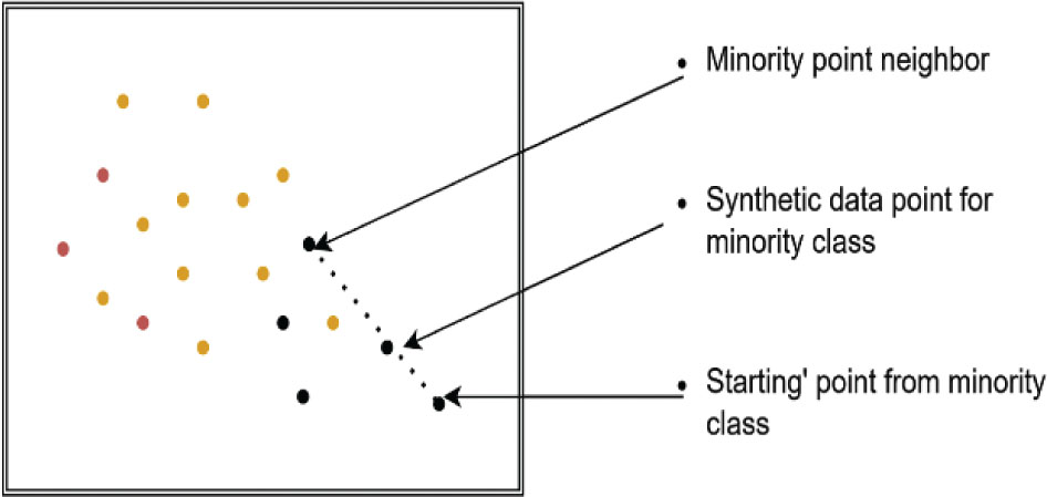
Figure 3:
SMOTE algorithm for a single iteration. SMOTE, synthetic minority oversampling technique.
Despite having more advantages than ROS, SMOTE suffers from a few disadvantages [33], such as ignoring the majority class by focusing on minority class instances, disturbing the original data distribution, because of which variants of SMOTE were developed with some improvement, as shown in Figure 4.
i) Borderline-SMOTE: Han et al. [34] introduced minority oversampling methods named borderline-SMOTE1 and borderline-SMOTE2, in which oversampling of minority samples only near the borderline was done. The authors proved the improvement of borderline SMOTE over simple SMOTE in terms of F-value and true positive rate. The problem is that it only improved the performance of the worst-performing classifier but did not improve the overall classification performance [33].
ii) Safe-Level-SMOTE: Bunkhumpornpat et al. [35] presented a technique, Safe-Level-SMOTE, as a solution for the class imbalance problem, which carefully over-samples the data. Unlike SMOTE or Borderline-SMOTE, which may generate synthetic instances in noisy or overlapping regions, this approach ensures that all synthetic samples are generated within safe regions. Each synthetic instance is created near the “safe level,” defined by the number of positive instances among its K-nearest neighbors. By focusing generation in these high-confidence areas, the method inherently avoids noisy boundaries and reduces the risk of introducing ambiguity. As a result, it enhances the quality of synthetic data and leads to more robust classifier performance compared to simple SMOTE or Borderline SMOTE.
iii) Adaptive Synthetic Sampling (ADASYN): ADASYN [36] is an adaptive synthetic sampling approach that improves imbalanced dataset learning in two ways: i) reducing the bias due to class imbalance and ii) adaptive shifting of classifiers’ decision boundary towards the minority class, which is harder to learn. Since minority class instances with fewer neighboring minority samples are generally more challenging for classifiers to learn, the method applies a weighted sampling strategy that reflects the learning difficulty of each instance. Specifically, it allocates higher weights to harder-to-learn samples with fewer same-class neighbors and lower weights to easier instances. As a result, complicated minority examples generate more synthetic samples, whereas simpler instances contribute less to the creation of synthetic data.
Like SMOTE, ADASYN creates fake samples along the path segment that links examples of the minority class. ADASYN uses a local density distribution to adaptively determine how many synthetic samples to create for every minority scenario. This adaptive mechanism ensures that more synthetic data is generated for harder-to-learn instances—those located in sparsely populated regions—while fewer samples are created for well-represented examples. As a result, the augmented dataset more accurately reflects the underlying distribution and encourages the classifier to focus on the more challenging decision regions.
iv) K-means SMOTE: Douzas et al. [37] proposed a new technique to handle class imbalance by combining SMOTE with the K-means clustering algorithm. Most of the old SMOTE techniques were complex and noise-generating. K-Means SMOTE is a three-phase oversampling technique that incorporates clustering into the sample generation process to address the imbalance in class. First, the K-Means algorithm is applied to partition the dataset into clusters. In the second phase, a filtering mechanism is employed to discard clusters containing a low proportion of minority class instances, as these clusters are less informative for synthetic sample generation. Furthermore, the density of minority class samples within each retained cluster informs the allocation of synthetic instances: clusters exhibiting lower minority class density are assigned a greater number of synthetic samples to address class imbalance more effectively. Subsequently, the SMOTE algorithm is applied within each selected cluster to generate synthetic minority instances, leveraging the local data distribution to preserve underlying structure. Experiments proved that the K-means SMOTE handles class imbalance between and within classes more effectively without the generation of noise. The algorithm gives better results on geometric mean, recall, and F1-score.
Cluster-based oversampling: Jo [38] addressed the issue of performance degradation in classifiers not only because of class imbalance but also resulting in small disjuncts due to imbalanced data. Experiments proved that the classifier gave superior performance to solutions to the class imbalance problem. First, clusters of each class were made separately, and then ROS was performed cluster by cluster. This technique rectifies two imbalances simultaneously: one is between-class imbalance, and the other is within-class imbalance. All clusters, with the exception of the largest, are randomly oversampled for the majority class clusters until their total number of observations equals that of the cluster with the greatest number of data points [39]. The minority class clusters are then randomly oversampled until each cluster includes m/N samples, assuming m as the number of instances of the majority class and N as the number of minority class clusters. This oversampling is the same as that of K-means SMOTE, with differences in a few aspects: K-means SMOTE relies exclusively on the K-means clustering technique and applies clustering across the entire dataset without separating classes. In contrast, cluster-based oversampling offers greater flexibility by allowing the user to choose any clustering algorithm and perform clustering separately for each class. Additionally, K-means SMOTE employs the SMOTE algorithm for generating synthetic samples, whereas cluster-based oversampling uses ROS to balance the class distribution. All the methods except ADASYN neglect the original data distribution, which is highly difficult to estimate.
GMMs: GMMs are probabilistic models. They assume the data, with its own mean and covariance, is derived from a finite number of Gaussian distributions. The model estimates both the parameters of these Gaussian components and the mixing weights, enabling it to capture complex, multimodal data distributions [40]. The objective of GMMs is to estimate the parameters that define both the mixing proportions and the underlying Gaussian components from the observed data. This estimation is typically performed using the Expectation-Maximization (EM) algorithm, a widely used iterative method. The EM approach alternates between the Maximization (M) phase, which modifies the model parameters to maximize the expected log-likelihood of the observed data, and the Expectation (E) step, which calculates the posterior probability of the latent variables given the current parameter values. Through this iterative process, the EM algorithm converges to a set of parameters that locally maximize the likelihood of the data under the GMM. GMMs are generative in nature and can create synthetic data by sampling from the learned distribution. To make sure that the new data closely resembles the real data, synthetic data points are created from the learnt distribution by randomly choosing a component based on the mixing weights and sampling from the matching Gaussian distribution. The only drawback is that GMM always considers a mixture of Gaussians to represent the correct data, which is not always true. A comparative analysis of the described standard and statistical methods, along with deep learning methods, is given in Table 1.
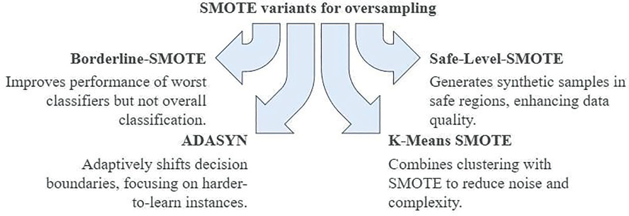
Figure 4:
SMOTE variants. SMOTE, synthetic minority oversampling technique.
Table 1:
Comparative analysis of SDG methods
| Method | Mechanism | Privacy | Evaluation metrics | Pros | Cons |
|---|---|---|---|---|---|
| ROS/RUS | ROS duplicates the minority class, and RUS removes the majority of the samples | No direct privacy guarantees | Classification accuracy, recall, F1 | Simple, ROS keeps the majority intact | RUS discards useful data, ROS risks overfitting |
| SMOTE | Interpolates between minority neighbors | No direct privacy layer | Classifier metrics (F1, recall) | Reduces bias | Ignores the majority class |
| Borderline-SMOTE | Generates samples near the decision boundary | No direct privacy | F-value | Targets hard-to-classify regions | Helps the worst classifier only |
| Safe-Level-SMOTE | Synthesizes only in “safe” neighborhoods (k-NN density) | No direct privacy | Robustness in the classifier metrics | Reduces noise, avoids overlaps | May under-cover rare but valid extremes |
| ADASYN | Adaptive sampling – more for sparse/minority regions | No direct privacy | ML metrics - recall, F1 | Focuses on hard-to-learn samples | Amplifies outliers in sparse areas |
| K-means SMOTE | Cluster data, filters clusters, and then applies SMOTE inside clusters | No direct privacy | Recall, F1 | Reduces noise, good for within and between class imbalance | Sensitive to clustering choice (k value) |
| Cluster-based oversampling | Per-class clustering, then oversample (ROS) each cluster | No direct privacy | Classifier performance | Fixes between and within imbalance, flexible | Uses ROS, not generative |
| AE | Encode–decode; reconstruct input | Indirect privacy via generative process | MSE, ML efficacy | Simple neural generative model | Weak latent representation, poor sample quality |
| VAE | Probabilistic latent space + KL divergence regularization | Improves privacy by sampling latent space | Reconstruct ion loss + KL, utility metrics | Principled latent representation, good quality | May blur/shrink modes, tuning complex |
| GAN | Generator–discriminator adversarial learning | Privacy by design; vulnerable if overfitted | Fidelity (KL, Wasserstein), utility (ML accuracy, F1) | Produces highly realistic samples | Training instability, mode collapse, vanishing gradients |
| TGAN | LSTM generator for continuous/categorical, MLP discriminator w/minibatch diversity | No explicit privacy, but avoids direct data use | Accuracy, F1, correlation metrics | Captures correlations, handles mixed data | Instability, imbalance not directly handled |
| CTGAN | VGM normalization + conditional generator | Same as GAN (synthetic by design) | Likelihood fitness, ML efficacy | Handles non-Gaussian continuous, imbalanced categorical | Complex, still inherits GAN pitfalls |
| TabFairGAN | WGAN-GP with fairness constraint; Gumbel-Softmax for categorical | Adds fairness constraints alongside privacy | Accuracy, F1 | outperforms TGAN/CTGAN for fair data | Possible trade-off: fairness vs. fidelity/utility |
[i] AE, autoencoders; CTGAN, conditional tabular adversarial network; GAN, generative adversarial networks; MSE, mean-squared error; ROS, random oversampling; RUS, random undersampling; SDG, synthetic data generation; SMOTE, synthetic minority oversampling technique; TabFairGAN, fair-tabular data generation with generative adversarial networks; TGAN, tabular generative adversarial networks; VAE, variational autoencoders; VGM, variational Gaussian mixture; WGAN-GP, Wasserstein GAN with Gradient Penalty.
b. Deep learning methods
Deep learning methods are used while generating new data instances, so the category is named as deep learning methods. These are difficult to interpret and understand as they are complex methods. Autoencoders (AE) and GAN are two classes of generative models. They have many variants, but it is not possible to cover all of them, so only a comprehensive overview of the techniques is covered in the literature.
b.i. AE
AE [41] are feedforward neural networks. The encoder and decoder are two parts of this neural network. The encoder compresses high-dimensional data to low dimensions, while the decoder decodes compressed data into its original form, as shown in Figure 5. An AE not only learns the input data, but it also copies the input samples approximately and generates a copy of the data that resembles the original data. The problem with AE is that there is no standard definition regarding data point distribution in latent space. So, we cannot determine whether the generated data is possible original data. Also, data points within the same class may have significant gaps in latent pace, leading to poor data generation. VAEs were developed as a solution to these AE problems.
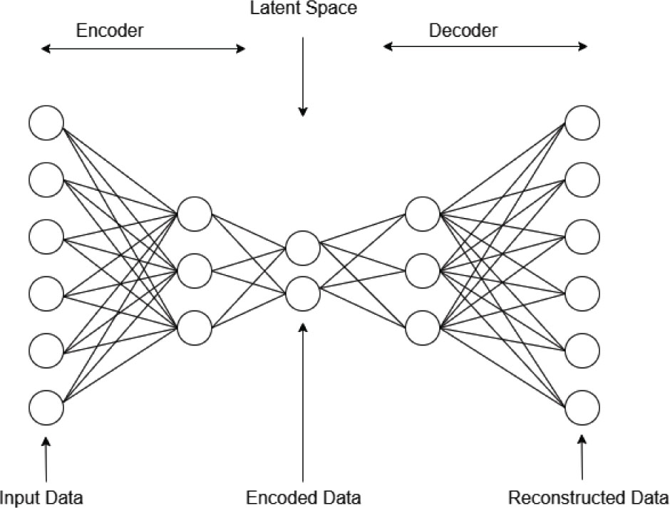
Figure 5:
Basic architecture of AE. AE, autoencoders.
VAE was first proposed by [7], which is an improved version of an AE with a few changes in the loss function and the encoder. A continuous, probabilistic representation of the latent space is encoded by VAEs.
This makes it possible for a VAE to employ variational inference to produce new data instances that closely resemble the original input data, in addition to precisely reconstructing the original input. For each latent variable in training data, VAE builds vectors named the mean vector and the vector of standard deviation. These vectors represent a range of possibilities for a given attribute with its expected variance. By taking this random sampling into consideration, VAE synthesizes new data that resembles the original data, which will be within the range of possibilities.
VAE uses reconstruction loss, such as mean-squared error or cross-entropy loss, to measure the difference between the original input and the output from the decoder. For more accurate reconstruction in latent space, some gradient descent optimization over the parameters of the encoder network will be performed, and the reconstruction error will be reduced. However, along with reconstruction of the original input, VAE targets a new sample generation for which one additional regularization term called Kullback–Leibler divergence (KL divergence) was incorporated. Adding KL divergence helps in reducing the gap between data points in the latent space and ultimately helps in generating a better framework for SDG. Islam et al. [42] used VAE to generate accident data. The author did experiments to compare VAE with SMOTE and ADASYN, and the results proved that VAE performs better than both and gives good classification metrics.
b.ii. GAN
Goodfellow et al. [6] proposed a GAN architecture for the first time in 2014, which has evolved till now and is capable of writing, painting, and composing. We will see GAN in terms of tabular data generation in this study, as it has many flavors intended for every work.
Generator G and discriminator D are two main functioning models of GANs, as shown in Figure 6. Generator (G) is used to produce synthetic samples that approximate the actual data distribution, generating outputs that are similar statistically but not identical to the real data, thereby avoiding mere replication of training examples. In contrast, discriminator D is tasked with distinguishing between real samples drawn from the actual dataset and fake samples produced by G. Through this adversarial process, both models improve over time: G becomes better at generating realistic data, while D becomes more accurate at classification. Although neural networks are commonly used to implement both G and D due to their expressive power, the framework is not limited to neural architectures; in principle, any differentiable function approximator can be employed.
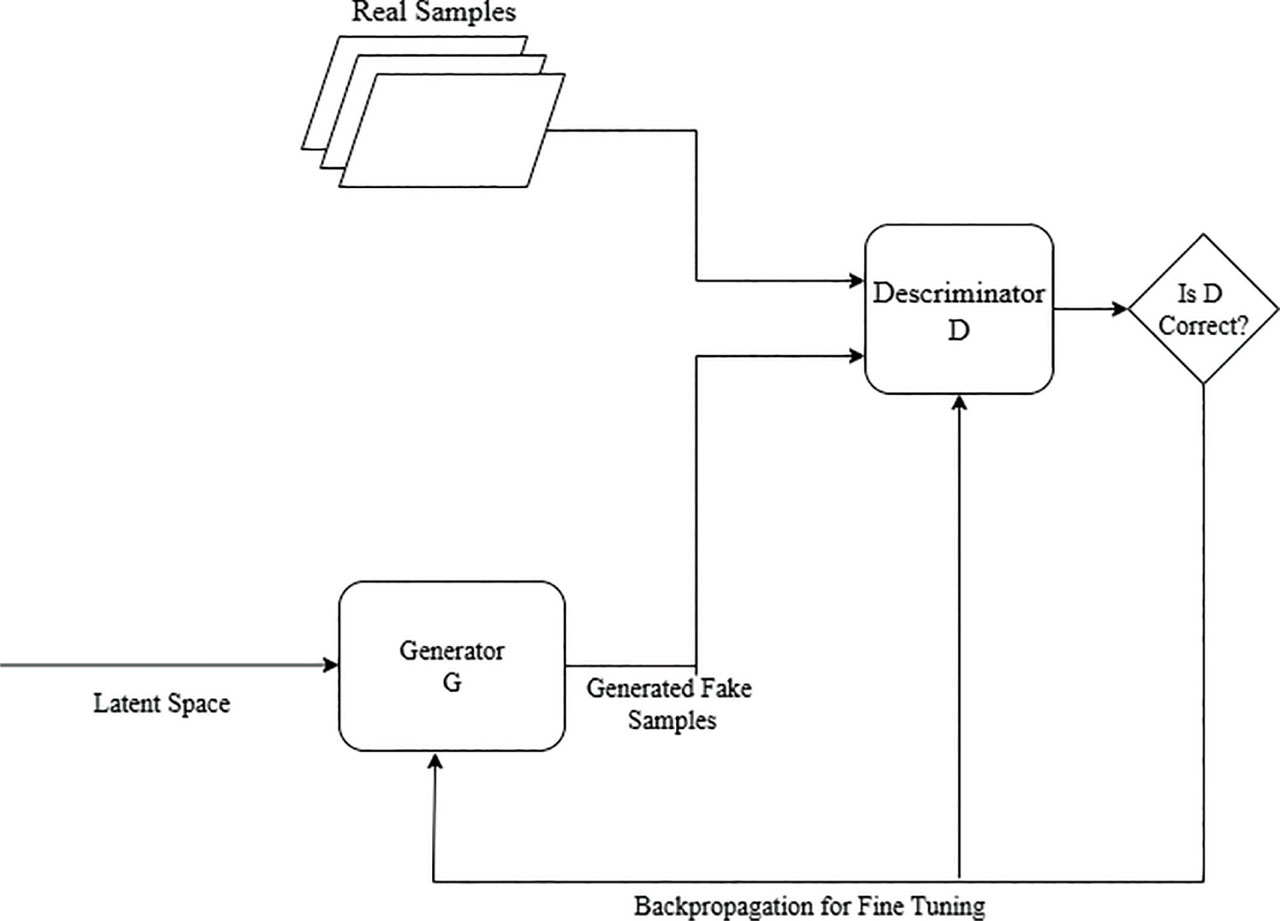
Figure 6:
GAN architecture. GAN, generative adversarial network.
Training for the discriminator and training for the generator were conducted independently. Discriminator is trained with original data points and data points generated from the generator G. It gives a probability from 0 to 1 and indicates whether the data belongs to original data or synthetic data. While the generator G is given random noise as input, called the latent space, from a MVND. The output from G has the same features as the input, but no verification exists there. So, the generator is provided with a loss function value, usually binary cross-entropy, which is the difference between the actual value and the computed probability.
Given the output from the discriminator, i.e., the loss function as input to the generator, it tries to improve itself by generating examples resembling the real data and ultimately tries to fool the discriminator. Along with this, discriminators also improve the identification of real and fake data.
Main drawbacks: GAN also carries some disadvantages, which are neither domain-specific nor dependent on any GAN architecture. A few of these problems include the hyperparameter tuning problem, the vanishing gradient problem, the mode collapse, and the uninformative loss. GANs have a significant number of hyperparameters that can be tuned to improve their performance. However, it results in a significant amount of time being required for training and high resource utilization.
The vanishing gradient problem occurs when the gradients used to update weights and generator training become too small. It happens when the discriminator becomes too good at differentiating between original and generated data. This leads to failure of generator training.
Mode collapse is a common issue encountered in GANs, where the generator produces a limited variety of outputs, often generating samples that are very similar to each other. Instead of capturing the full diversity of data distribution, the generator focuses on a few modes, effectively ignoring others. As a result, it fails to generate samples that represent the broader data space. This limited diversity can confuse the discriminator, as it repeatedly sees only a narrow subset of generated samples, making it less effective at distinguishing between real and synthetic data.
Training of generators is difficult to monitor because there is no correlation between the quality of the generated output and the loss. The generator loss is typically referred to as binary cross-entropy, and it does not provide any kind of information. These are a few disadvantages encountered in GAN data generation.
V. GANs for Tabular Data Generation
The majority of the data generation tasks using GAN were performed on image generation, but most of the datasets are numeric in nature. The same GAN architecture used for image generation cannot be used for tabular data generation, as tabular data has its own properties. Numerical data is a combination of categorical and continuous data. Categorical data is imbalanced most of the time. Also, features of numerical data may have a non-Gaussian distribution and multiple modes. To avoid these problems, three GAN architectures - Tabular GAN (TGAN), conditional tabular adversarial network (CTGAN), and fair-tabular data generation with GAN (TabFairGAN) can be used for tabular data generation. As this study is intended to study tabular SDG, which is not much disseminated in the literature, the details of the techniques are provided below.
a. TGAN
Xu and Veeramachaneni [43] proposed TGAN for the first time in 2018 to generate tabular data with categorical and numeric values. Adding the power of deep neural networks, TGAN can generate high-quality tabular synthetic data. The generator and discriminator are the two main parts of TGAN, and they work together within a GAN framework.
A generator based on an long short-term memory network, which is excellent at producing sequential data, serves as the foundation for the generator. It can handle multimodal distributions since it produces both the cluster vector and the value scalar for continuous variables. It ensures realistic one-hot encoded outputs for categorical variables by generating a probability distribution over potential categories.
A multilayer perceptron (MLP) serves as the discriminator, separating synthetic data from actual data. To improve training and avoid mode collapse, it makes use of strategies, such as diversity metrics and minibatch discrimination. The working architecture of TGAN is shown in Figure 7.
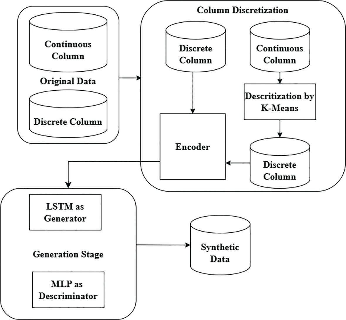
Figure 7:
TGAN for generating two discrete and two continuous variables. LSTM, long short-term memory network; MLP, multilayer perceptron; TGAN, tabular generative adversarial networks.
In the study by Xu et al. [43], the authors evaluated TGAN, and experiments proved that TGAN is successful in capturing the correlation between two variables. Also, evaluation in terms of F1 score and accuracy proved that TGAN performs well when machine models are trained with real and synthetic data.
b. CTGAN
As an improvement in TGAN, Xu et al. [44] proposed CTGAN in 2019. Like TGAN, CTGAN was explicitly designed to synthesize mixed (numeric and discrete) data. Along with preserving the correlation between two columns, it also preserves the joint distribution between all columns. Continuous data features in the dataset often follow a non-Gaussian multimodal distribution. To capture this, CTGAN uses mode-specific normalization. Instead of GMM, it uses a Variational Gaussian Mixture model, which represents continuous feature value as a one-hot encoding vector to represent its sample mode and one scalar that represents the value is normalized according to the mode.
In case of synthesizing categorical data, CTGAN faces two main challenges: one is the sparsity of the one-hot encoded vector, and the second is the imbalancing associated with categorical features. The author employed a conditional generator, which creates synthetic rows that rely on any of the categorical columns, to address imbalanced categorical columns. Also, a sample-by-sample training technique was introduced to examine every discrete value in the dataset uniformly. The CTGAN model is shown in Figure 8.
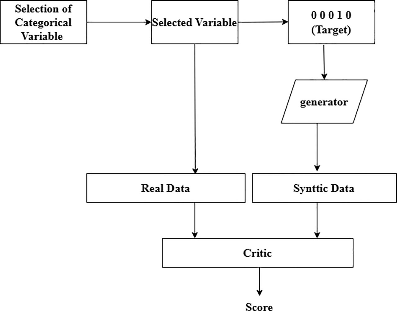
Figure 8:
CTGAN model. CTGAN, conditional tabular adversarial network.
To evaluate the performance of CTGAN, the author used a likelihood fitness metric for simulated data evaluation. To evaluate real data performance, ML efficacy is used, as we are unaware of the distribution of the data. In the case of real data, CTGAN outperformed other generative models, such as TableGAN and Medical Generative Adversarial Network (MedGAN). However, in the case of simulated data, it performed relatively better than other models in terms of the likelihood fitness metric. Finally, the author performed an ablation study to evaluate the utility of the conditional generator, mode-specific normalization, and sample-by-sample training. The results showed that they are a very important factor in generating high-quality tabular data.
c. TabFairGAN
To generate tabular data, Rajabi and Garibay [45] introduced TabFairGAN. The model contains two stages: first, the TabFairGAN model was trained to produce data that resembled the original data. The value function was modified in the second phase to include fairness restrictions, allowing the network to keep learning to produce data that is accurate and fair. As the tabular dataset contains both numerical and categorical variables, categorical values were represented by a one-hot vector. Numerical columns sampled from multimodal distributions were transformed by the author using a quantile transformation method.
The architecture of the TabFairGAN model is shown in Figure 9. The author designed a network as Wasserstein GAN (WGAN) with a gradient penalty, where the generator takes a latent variable as input from a MVND and generates sample data. A critic in a model receives that sample data as input. The generator may produce synthetic data that looks like actual data after both the critic and the generator are properly educated. A fully connected first layer with the Rectified Linear Unit (ReLu) activation function is present in the generator. Several vectors were concatenated to form a hidden layer that generates data like the original data. A fully connected layer with ReLu activation function was implemented for numerical variables, while multiple fully connected layers with Gumbel SoftMax activation were used for discrete variables to generate a one-hot vector. Resulting nodes are then concatenated to feed them as an input to the critic network. Critic is a fully connected layer network with LeakyReLU activation function. Author [45] proved through experiments that TabFairGAN is more effective than TGAN and CTGAN on ML models, MLP, logistic regression, and decision trees in terms of accuracy and F1 score. So, it is quite an effective way to generate tabular data like original data. As shown in Table 1, all the methods used for SDG differ not only in terms of mechanism but also, they differ in privacy aspects and evaluation metrics.
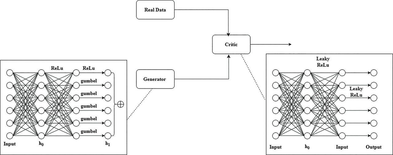
Figure 9:
TabFairGAN Architecture. Image taken from [45]. TabFairGAN, Fair-tabular data generation with generative adversarial network.
VI. Quality Check Metrics for Generated Data
Assessing the quality of generated data is a critical task. If synthetic data can capture the same distribution as the parent distribution, then it may possess the same quality. The extent to which the generated tabular data matches the real data is determined by several defined measures that are used as benchmarks when evaluating the quality of continuous synthetic data. This section focuses on the evaluation of tabular synthetic data.
The simplest method for evaluating continuous data is a comparison of its basic statistics. If the statistics (mean, median, and standard deviation) of generated data match the original data, then the synthetic data is said to be like real data. However, as stated by a statistician [46], as data distributions may be different, this can be misleading.
As a solution, a few advanced statistical methods that compare the probability distribution can be used as predefined metrics. Each of which is described below:
KL Divergence: To measure the difference between two continuous distributions, KL divergence [47] calculates the probability distribution (ranges from 0 to positive infinity) between two values. If the value is close to 0, then the distributions are close to each other, while a value near infinity indicates similarity between the actual and fake data. It is a powerful technique for assessing fidelity when synthetic data is supposed to mimic the fine-grained statistical characteristics of real data, since it is especially helpful in identifying minute variations in distributional density.
Wasserstein Distance: It is frequently used to calculate the distance between two continuous data probability distributions, which indicates the amount of change required to bring one distribution into line with the other. Again, a small value indicates high similarity, and a large value indicates dissimilarity [48]. This metric offers a robust measure of fidelity and potential downstream utility for tabular data by quantifying the alignment between real and synthetic distributions within continuous feature space.
Energy Distance: The Energy Distance is the difference between two different probability distributions in continuous space. Similar to the Wasserstein distance and the KL divergence [47], the Energy Distance is a statistical indicator of distributional dissimilarity. Lower values of the Energy Distance indicate that the distributions are more similar, while higher values reflect greater dissimilarity [49]. Handling multimodal and high-dimensional data is a strength of this metric, as it considers both the spread of distribution and mean to extend comparison. This technique is useful to enhance the fidelity and generalizability of data by preserving complex distributional structure.
Maximum Mean Discrepancy (MMD): A statistical metric, MMD, is used to evaluate the separation between two probability distributions. When two samples are taken from different distributions, it calculates the most significant difference between their mean embeddings. It is useful in detecting non-linear distributional discrepancies in data. Capturing structural differences in data, it ensures fidelity during evaluation. A larger MMD value indicates greater dissimilarity, while a smaller value signifies higher similarity between the distributions [50].
Plotting the data using different graphs, such as boxplots, histograms, and violin graphs, is the simplest way to check data distributions in a visualized form. A Q-Q plot is used to plot two probability distributions against each other. It showcases the similarity between two distributions by plotting their quantiles against each other. Plotting thousands of data points is an expensive way of assessing data quality, so a few other ways can be used.
Based on the ML model performance trained with synthetic data, ML efficacy becomes one more quality evaluation metric for generated data. To check ML model performance, data D is split into train (Dtrain) and test (Dtest) data. The model is then trained with Dtrain and Dsynth data and evaluated on Dtest data, as shown in Figure 10.
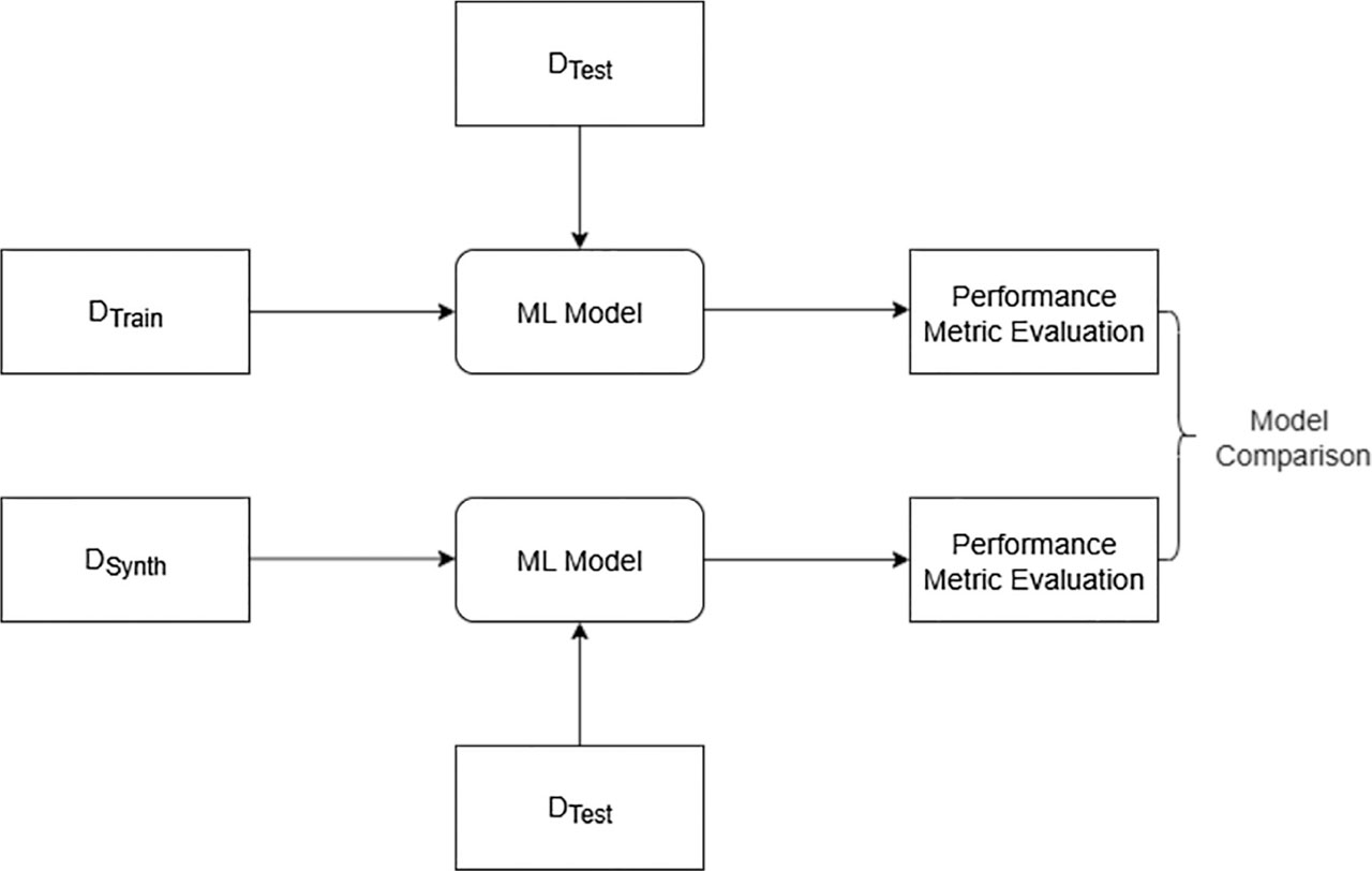
Figure 10:
ML efficacy. ML, machine learning.
If a ML model trained on generated data achieves metrics—such as F1-score, precision, recall, and accuracy—comparable to those obtained when trained on real data, it shows that the underlying point distribution of the original data is successfully captured by the created data. This assessment metric is used by [43] and [44] to measure the performance of the CTGAN and TGAN architectures.
SDG improves ML efficacy by several mechanisms, such as the generation of more diverse data and an increase in data volume, which mitigates data imbalance and at the same time develops a more generalized model [28]. Along with this, synthetic data allows inclusion of rare and underreported data instances in real-world data to prepare a more robust model. Third, synthetic data ensures data privacy by maintaining confidentiality and providing alternatives to real data for model training [44]. Synthetic data is applicable to domains where data availability is limited, needs privacy, and data collection is difficult as well as costly. Noticeable applications include medical diagnosis via imaging, where synthetic data can generate medical images to avoid data scarcity, and finance, where synthetic data maintains privacy along with the injection of diverse transaction conditions for fraud detection. Though generated data improve model performance, validation of the model with real data is essential in order to ensure model reliability [28].
This section focuses on examining different synthetic data evaluation metrics. It is always better to utilize a combination of any two instead of any one, for better assessment. Evaluating the synthetic data depends on the problem to solve and is a challenging task. Sometimes, different metrics need to be used in case of the same problem with different scenarios. Synthetically generated data may cover distribution, but fails to achieve feature dependencies. So, focusing on a single metric may violate others, e.g., focusing much on fidelity may result in data memorization with privacy risk. Here are a few use cases with the benefit of metric combination shown in Table 2:
Table 2:
Metric combination with SDG methods use cases
| Use case | Synthetic data use | Metric combination used with experimental details |
|---|---|---|
| Generation of synthetic data for medical diagnosis [51] | To preserve rare disease cases without copying patient personal information, as rare disease cases are very few in number and generate a high data imbalance, which negatively affects model performance. | The author generated synthetic data using a GAN and measured statistical similarity between the original and generated data probability for each feature. Results with lower KL divergence proved high similarity, maintaining statistical properties of the original data. Diagnosis performance of the predictive model, trained on both (real and synthetic) data, was tested with accuracy and F1 score. Result shown less variation and minimal risk of individual identification. |
| Data Sharing [52] | Replication of data by maintaining its statistical distribution and no re-identification risk. Use of synthetic data ensured secure data exchange. | Synthetic data was generated using a GAN and the Gaussian Copula Method. Its quality was assessed based on statistical similarity and data distribution with the statistical distribution metric (MMD). It was observed that GAN gave the most satisfactory result by replicating the statistical structure of the original data. |
| To check the quality of generated data on the performance of predictive models, the model was trained with real data first to find basic performance metrics, such as accuracy, precision, and recall. In the second step, the model was trained with synthetic data, and in the final step, training was done with a combination of both. | ||
| Model tested on real test data to assess the overall performance of the model. Results showed that synthetic data better replicates correlations by giving better prediction results. |
VII. Challenges, Risks, and Future Scope
Generalization and Robustness: Preserving statistical properties of original data is a significant challenge in SDG [53]. Therefore, developing advanced methods to ensure the originality of data can be an area of focus.
Scalability: Scaling of generated data to larger datasets or diverse data is another challenge in SDG. As generated data may only mimic certain features of the original data. Also, unbalanced discrete columns and skewed continuous columns may not be correctly modeled [54].
Evaluation Metric and Utility: Ensuring reliable evaluation for assessment of generated data is an area of improvement in SDG, which poses an additional challenge of utility [55]. Because if synthetic data does not represent the underlying patterns of original data, then we cannot use generated data for analysis or model training.
Re-identification Risk: Zhang et al. [56] stated that, based on experimental results, partial synthetic data has high risk of vulnerability while fully synthetic data is protected from attacks of re-identification. More work is required in order to limit the re-identification risk. Risk associated with re-identification of synthetic data is still evolving. Currently, it is considered a secure way of data sharing as there is no direct linkage between generated data and original data.
VIII. Conclusion
This survey aimed to provide SDG methods and their evaluation metrics. In contemporary data science, SDG has become a game-changing technique that tackles important issues with bias reduction, privacy protection, and data scarcity. One of the major issues observed while conducting this survey is that very little literature is available on tabular data generation compared to image data. So, GAN with tabular data generation still has room for improvement. The study also highlights how crucial it is to use strong evaluation metrics when evaluating the overall quality of synthetic data. Each of these factors—fidelity, variety, utility, and privacy preservation—offers a different perspective on how effectively synthetic data replicates its real-world counterparts while upholding moral and legal requirements.
In summary, the creation of synthetic data serves as a spur for innovation as well as a replacement for actual data. It has the potential to improve decisions based on data while preserving privacy and equity if it is carefully designed and assessed.