
Table 1:
Cutting-edge studies on traffic sign detection implemented in Ecuador
| References | Model type | Description | Dataset | Results |
|---|---|---|---|---|
| [3] | CNN | Data augmentation and preprocessing techniques were employed to enhance model performance. Three models were developed and tested: a traditional neural network, a CNN without regularization, and a CNN with regularization | Dataset from public and manually collected pictures. It contains 5,322 images. | 91% accuracy on validation data and 81% on test data |
| [29] | CNN | Four well-established CNN architectures were employed. | Unknown sources | 98.6% accuracy, 99.30% sensitivity, a 99.63% AUC, a 98.89% AP, and a 99.42% F1 score |
| [7] | R-CNN | An object detection model based on the Faster R-CNN architecture was implemented, using ZF-Net as the backbone network for feature extraction. | The dataset comprises 52 classes, collected under various lighting conditions across multiple locations in Ecuador. | The evaluation of the model did not include specific quantitative performance metrics |
| [30] | R-CNN | Same as in [7] R-CNN without ZF-Net | The same dataset was used in [7] | The evaluation of the model did not include specific quantitative performance metrics |
| [31] | ELM | A two-stage multi-classification algorithm, based on ELM and HOG descriptor | Dataset from public and manually collected pictures. It contains 47,000 images. | 99.85% accuracy, 99.78 of sensitivity in the first stage. 96.71% accuracy, 94.16 of sensitivity in the first stage. |
| [32] | CNN | Dataset from public and manually collected pictures. It contains 37,500 images. | The evaluation of the model did not include specific quantitative performance metrics |
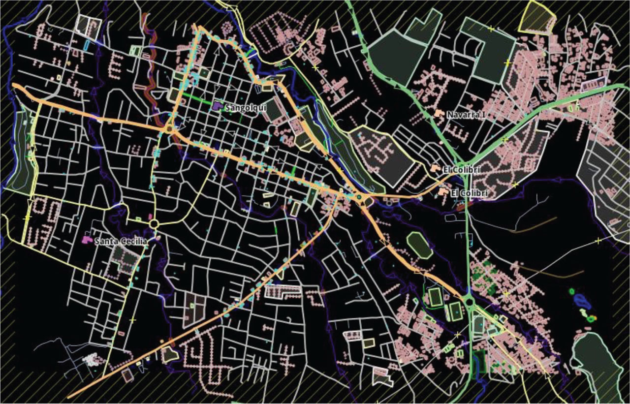
Figure 1:
Map of Sangolquí, Ecuador.
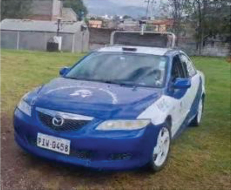
Figure 2.
Vehicle platform.
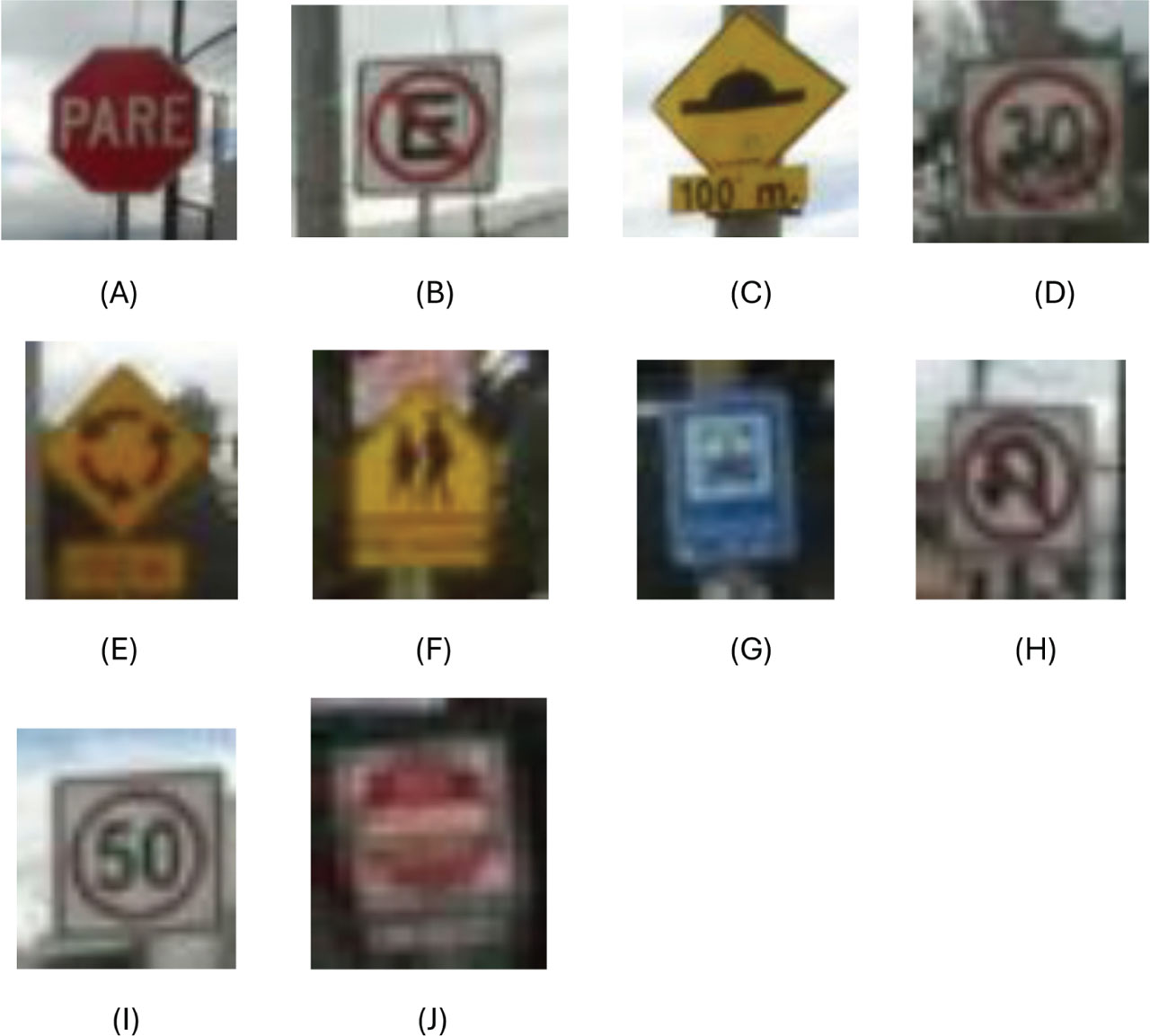
Figure 3:
(A) Ecuadorian stop, (B) no stopping or parking, (C) speed bump ahead, (D) 30 km/h speed limit, (E) roundabout ahead, (F) school zone (G) bus stop, (H) no U-turn, (I) 50 km/h speed limit, (J) no entry.
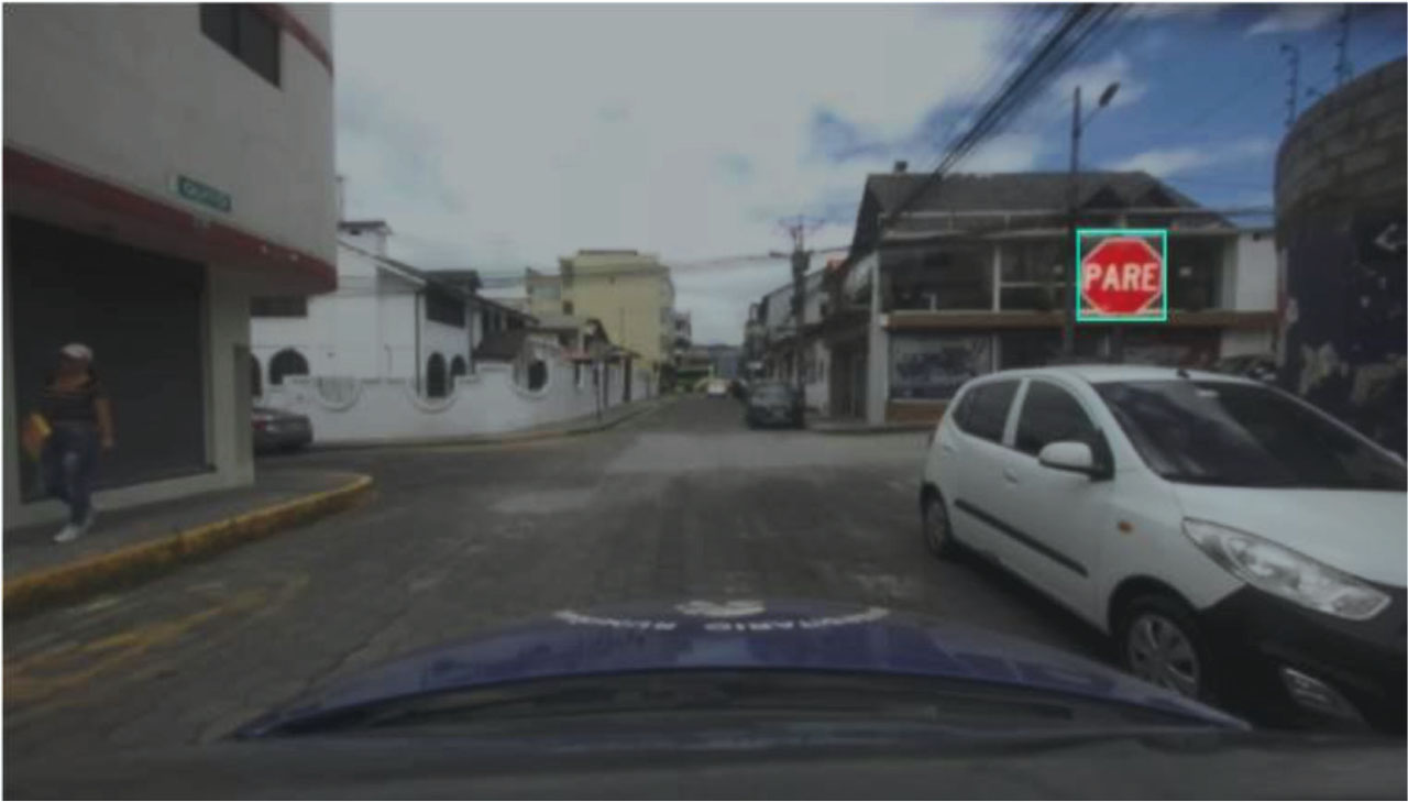
Figure 4:
Image annotation.
Table 2:
Features of YOLO models
| Features | YOLOv11 [34] | YOLOv12 [35] | YOLOv26 [36] |
|---|---|---|---|
| Architecture | Optimized CNN (C3K2, CSP-like) | Attention-centric (efficient attention, R-ELAN) | Simplified CNN + end-to-end NMS-free |
| Post-processing | Requires traditional NMS | Requires NMS | Native end-to-end without NMS |
| mAP COCO (approx. Variant) | ~51%–52% | ~53%–54% (v1 better in some reports) | ~53%–53.1% (slightly superior to YOLO11 in official benchmarks) |
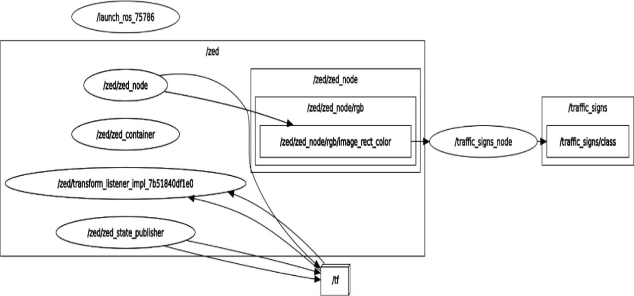
Figure 5:
RQT graph illustrates the communication between the zed 2i camera and the traffic sign detection node.
Table 3:
Computing infrastructure for model training
| Name | Type |
|---|---|
| CPU | CPU 4 cores |
| GPU | T4 |
| RAM | 16 GB |
| Framework | PyTorch |
Table 4:
Model training parameters
| YOLOv11 | YOLOv12 | YOLOv26 | |
|---|---|---|---|
| Epochs | 150, 200 | 150, 200 | 150, 200 |
| Batch size | 16 | 16 | 16 |
| Optimal algorithm | Adam | Adam | Adam |
| Model weight | YOLOv11n | YOLOv12n | YOLOv26n |
Table 5:
Performance metrics of the YOLOv11n, YOLOv12n, and YOLOv26n models at 150 and 200 epochs
| Models | Epochs | Precision | Recall | mAP50 | mAP50-95 |
|---|---|---|---|---|---|
| YOLOv11n | 150 | 0.69353 | 0.92976 | 0.96008 | 0.65295 |
| YOLOv11n | 200 | 0.69625 | 0.91667 | 0.94615 | 0.65097 |
| YOLOv12n | 150 | 0.70033 | 0.94868 | 0.99386 | 0.66485 |
| YOLOv12n | 200 | 0.9263 | 0.7375 | 0.88789 | 0.63377 |
| YOLOv26n | 150 | 0.8091 | 0.81977 | 0.896 | 0.63967 |
| YOLOv26n | 200 | 0.93036 | 0.63968 | 0.77258 | 0.55697 |
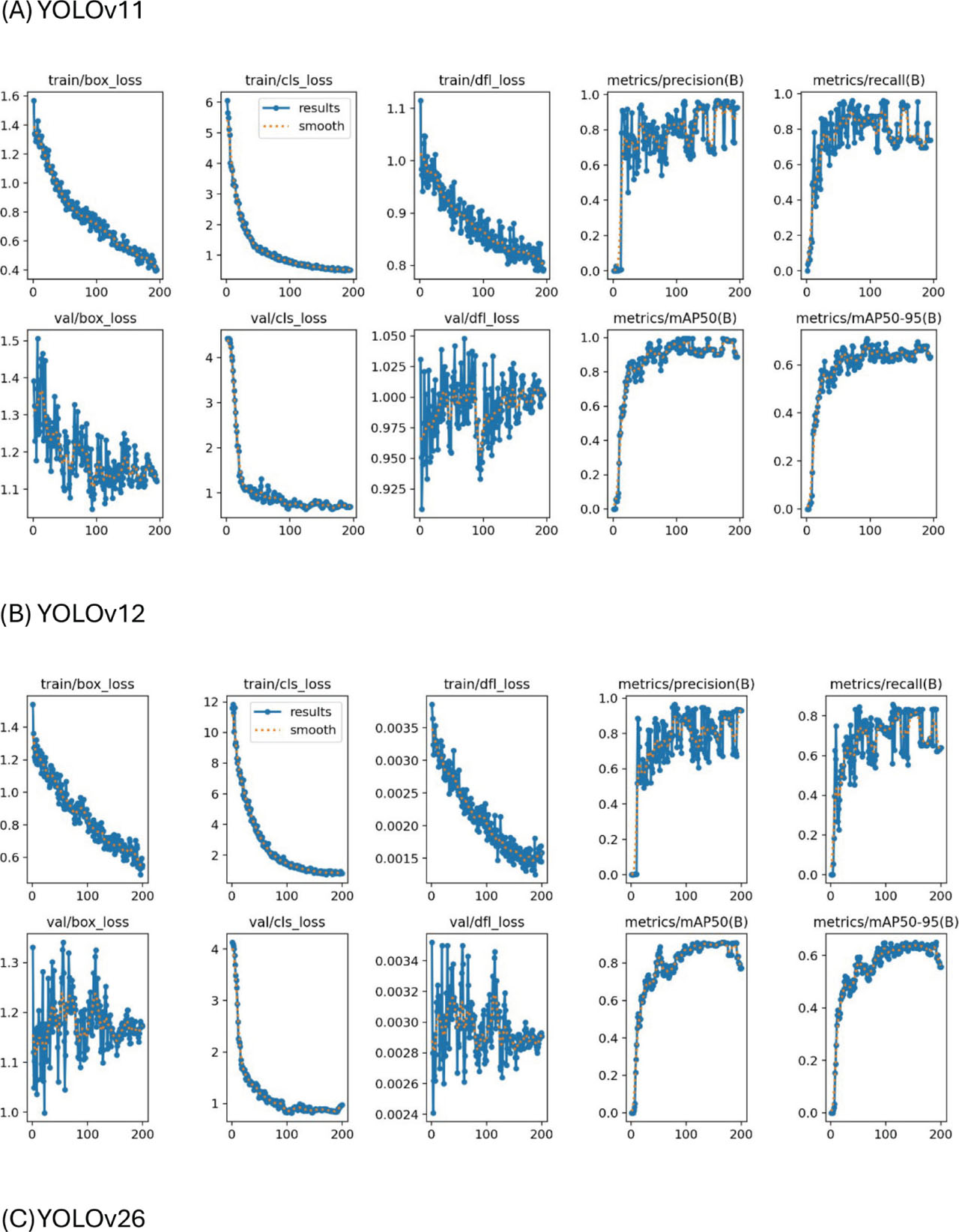
Figure 6:
The training and validation losses of YOLOv11 (A), YOLOv12 (B), and YOLOv26 (C).
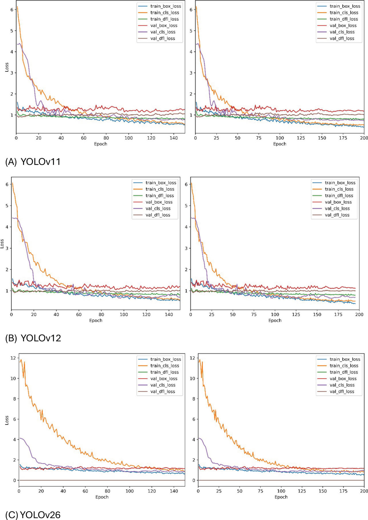
Figure 7:
Comparative analysis between the 150 and 200 epochs of YOLOv11 (A), YOLOv12 (B), and YOLOv26 (C).
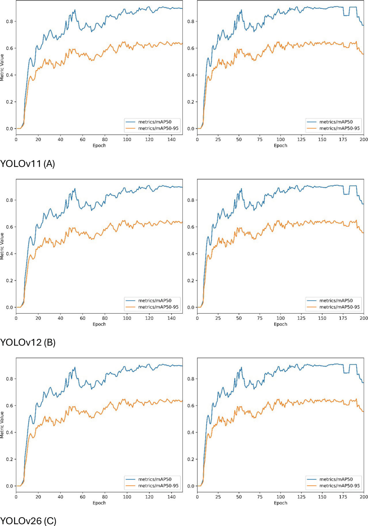
Figure 8:
Smoothed metrics for mAP@50 and mAP@50-95 over 150 epochs and 200 epochs of YOLOv11 (A), YOLOv12 (B), and YOLOv26 (C).
Table 6:
Changed training parameters of the YOLO models
| Parameter | Value |
|---|---|
| epochs | 200 |
| imgz | 640 |
| batch | 64 |
| lr0 | 0.01 |
| warmup_epochs | 3.0 |
| warmup_bias_lr | 0.1 |
| momentum | 0.8 |
| weight_decay | 0.0005 |
| optimizar | SGD |
| amp | True |
Table 7:
Performance metrics with changes to the YOLOv11n, YOLOv12n, and YOLOv26n models over 200 epochs
| Models | Epochs | Precision | Recall | mAP50 | mAP50-95 |
|---|---|---|---|---|---|
| YOLOv11n | 200 | 0.95611 | 0.72357 | 0.87374 | 0.60009 |
| YOLOv12n | 200 | 0.92965 | 0.75729 | 0.96251 | 0.65297 |
| YOLOv26n | 200 | 0.93036 | 0.63968 | 0.77258 | 0.55697 |
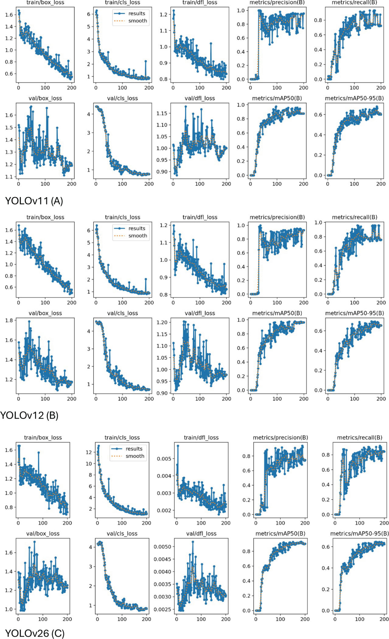
Figure 9:
The training and validation losses of YOLOv11 (A), YOLOv12 (B), and YOLOv26 (C) after the parameter change.
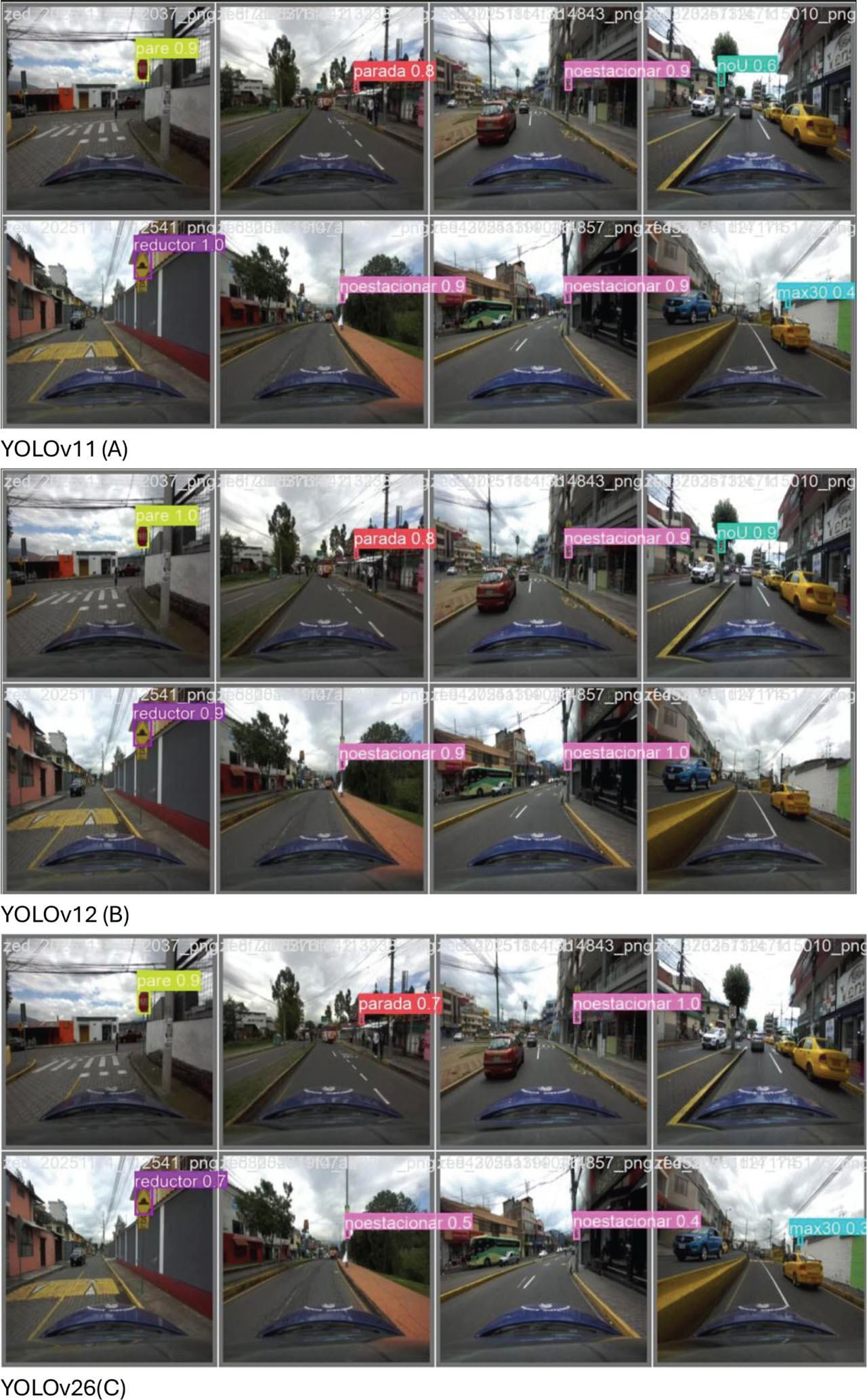
Figure 10:
Examples of traffic sign detections of YOLOv11 (A), YOLOv12 (B), and YOLOv26 (C).
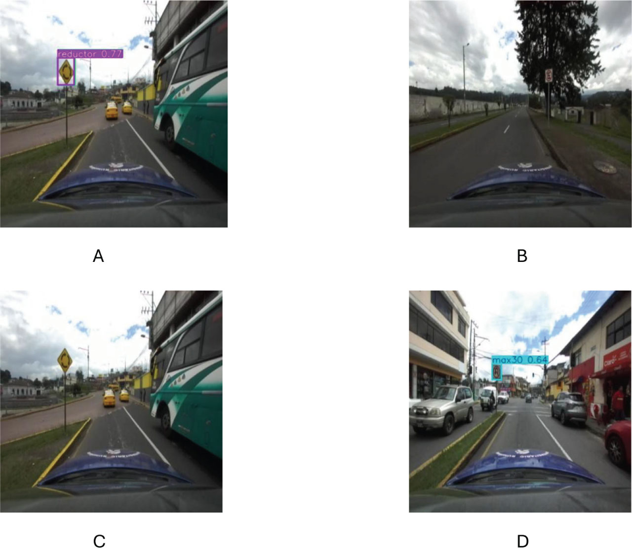
Figure 11:
Examples of FP (A,D) and FN (B,C). FN, false negatives; FP, false positives.