
I. Introduction
Autonomous vehicles have undergone rapid development in recent years, and perception systems play an important role in providing safe navigation in complex urban environments [1]. Reliable navigation involves critical tasks, and traffic signal detection remains a fundamental challenge in regions with diverse signaling standards and variable environmental conditions [2]. This problem is particularly acute in urban contexts in Latin American cities, where road safety issues are not a priority [3].
The integration of real-time object detection algorithms, such as YOLO [4, 5], has demonstrated high speed, architectural simplicity, and a better balance between accuracy and efficiency. However, many studies focus on datasets from North American or European contexts, which casts doubt on the performance of these models in regions such as Ecuador, where greater visual variability is observed [6,7,8]. Nevertheless, training these models requires robust hardware, which hinders the capability of computational resources [9].
Traffic sign detection systems on autonomous vehicle platforms face challenges in using devices, such as cameras and sensors, with limited sensitivity in low-light, backlighting, or nighttime conditions; diversity and ambiguity of signs; variability of the environment; integration with decision-making systems; and real-time processing. In this context, advanced driver assistance systems are a fundamental tool in mitigating existing risks. They also directly influence vehicle safety and compliance with traffic regulations in autonomous driving platforms [10,11,12]. Recent YOLO architectures focused on autonomous driving incorporate advances such as illumination-adaptive feature enhancement [13], 3D U-Net [14], attention-concentrated enhanced cross-stage partial network [15], dynamic cross-scale feature fusion module, and a dual-path downsampling convolution module [16]. These improvements enhance the models’ capabilities in detecting small objects, low-resolution urban scenes, and lighting conditions, including adverse traffic conditions.
A large number of traffic sign detection studies are based on reference data such as GTSDB [17], GTSRB [18], Belgium Traffic Sign Detection Dataset [19], LISA Traffic Sign Dataset, and GLARE [20] or TT100K [21], which are collected in moderately structured road conditions in Europe, Asia, or the USA. These datasets have accelerated the creation of new algorithms that have been trained and validated with high acceptance. However, Ecuadorian urban environments present challenges such as heterogeneous infrastructure, partial degradation of signage, inconsistent standards, and even diverse weather conditions. These factors can significantly affect the robustness of the models.
One of the technological tools in autonomous driving systems is stereo cameras, which help complement RGB-based object detection. The most widely used models, ZED [22] and Intel RealSense [23], are representative of typical experimental platform uses due to their real-time estimation capabilities, compatibility with ROS environments, and suitability for research prototypes.
This study analyzes efficiency by evaluating three YOLO-based models (YOLOv11, YOLOv12, YOLOv26) in detecting traffic signals in Ecuadorian urban environments. The hypothesis is that, although the models will demonstrate robust performance, their capability will vary depending on their traceability. To test this hypothesis, a dataset will be constructed using a ZED2i stereo camera to capture traffic signs in various scenarios in Sangolquí, Ecuador. The dataset includes vertical regulatory and informational traffic signs, which will be annotated and divided respectively for training, validation, and testing.
Most works use data from Europe, North America, or Asia. These datasets do not show the real problems found in Latin American cities. This is true for Ecuador, where road signs often show wear, vary in style, and face harsh weather. Previous local work focused on classical computer vision or convolutional neural network (CNN)-based approaches, with limited exploration of recent YOLO architectures and their comparative performance under real-world constraints.
Thus, this study fills a gap by testing new YOLO models. The models are trained and tested on local datasets representing real Ecuadorian city scenes. Furthermore, they are integrated into a real-time robotics system using robot operating system (ROS2) to enhance their practical applicability.
The article is organized as follows: Section II reviews related work. Section III details the methodology, including the construction of the dataset. Section IV presents the results and discussion. Section V presents the study’s conclusions.
II. Literature Review
Regional studies have demonstrated advances in object detection and recognition using YOLO-based architectures [24]. The YOLO family of models has been used by several authors for traffic sign detection in regional environments such as Brazil [25, 26], Peru [27], and Argentina [28]. However, the dataset used in these studies is not publicly available in accessible scientific repositories, which limits the reproducibility of the studies, one of the fundamental principles of scientific research. In many cases, the models have been partially trained using international datasets that do not represent the same visual characteristics. This negatively affects the accuracy and robustness of the systems in real environments. Nevertheless, to the best of the authors’ knowledge, previous studies on traffic sign detection in the Ecuador region have focused only on classical computer vision models.
Table 1 summarizes recent studies highlighting the algorithms used for traffic sign detection in the Ecuador region.
Table 1:
Cutting-edge studies on traffic sign detection implemented in Ecuador
| References | Model type | Description | Dataset | Results |
|---|---|---|---|---|
| [3] | CNN | Data augmentation and preprocessing techniques were employed to enhance model performance. Three models were developed and tested: a traditional neural network, a CNN without regularization, and a CNN with regularization | Dataset from public and manually collected pictures. It contains 5,322 images. | 91% accuracy on validation data and 81% on test data |
| [29] | CNN | Four well-established CNN architectures were employed. | Unknown sources | 98.6% accuracy, 99.30% sensitivity, a 99.63% AUC, a 98.89% AP, and a 99.42% F1 score |
| [7] | R-CNN | An object detection model based on the Faster R-CNN architecture was implemented, using ZF-Net as the backbone network for feature extraction. | The dataset comprises 52 classes, collected under various lighting conditions across multiple locations in Ecuador. | The evaluation of the model did not include specific quantitative performance metrics |
| [30] | R-CNN | Same as in [7] R-CNN without ZF-Net | The same dataset was used in [7] | The evaluation of the model did not include specific quantitative performance metrics |
| [31] | ELM | A two-stage multi-classification algorithm, based on ELM and HOG descriptor | Dataset from public and manually collected pictures. It contains 47,000 images. | 99.85% accuracy, 99.78 of sensitivity in the first stage. 96.71% accuracy, 94.16 of sensitivity in the first stage. |
| [32] | CNN | Dataset from public and manually collected pictures. It contains 37,500 images. | The evaluation of the model did not include specific quantitative performance metrics |
The studies in Table 1 demonstrate, in a comprehensive manner, the need created by a set of images due to the absence of regional public scientific repositories. Another aspect is the specific adaptations for each region, as these are crucial for the optimal performance of the proposed models.
III. Materials and Methods
a. Definition of the dataset
The dataset used in this study contains 640 images and is available at https://doi.org/10.6084/m9.figshare.31943658. Given that no regional data is publicly available, data collection was carried out in Sangolquí, as shown in Figure 1, a growing urban area in the Rumiñahui canton, Pichincha province, Ecuador. The data accurately represent the real conditions of traffic signals in Ecuadorian urban environments.
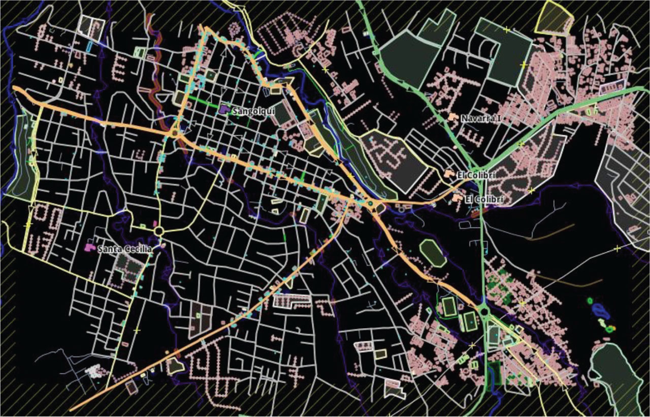
Figure 1:
Map of Sangolquí, Ecuador.
The images were collected in different sectors, including residential neighborhoods, school zones, and signal intersections. These locations were selected because they represent variable and diverse traffic density within the urban environment.
The images were captured using the ZED-2i camera. The camera was installed on top of a vehicle platform. This vehicle is part of a research project on autonomous driving, as shown in Figure 2. The vehicle is also equipped with a RoboSense RS-LiDAR-16 sensor for 3D environment detection and a SparkFun u-blox ZED-F9P GPS-RTK-SMA receiver module for high-precision RTK positioning. The core of the system is an ASUS VivoBook laptop, equipped with an Intel® Core™ i7-10750H @ 2.60 GHz processor and an NVIDIA TU117M GPU. The operating system used is Ubuntu 22.04 LTS, as the basis for the ROS2 Humble distribution.
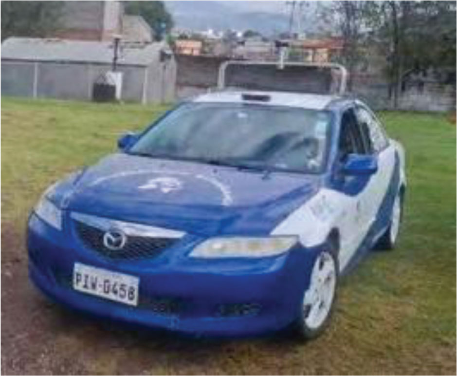
Figure 2.
Vehicle platform.
Data were collected under different environmental conditions to ensure data robustness. In addition, images were captured from different viewing angles and distances to simulate different realistic driving orientations.
The National Transit Agency is the public body in Ecuador responsible for regulating road safety. In this context, there are approximately 150–200 traffic signs. This work was limited to 10 main categories, each category having between 50 and 60 instances. The categories are: Ecuadorian Stop, No Stopping or Parking, Speed Bump Ahead, 30 km/h Speed Limit, Roundabout Ahead, School Zone, Bus Stop, No U-Turn, 50 km/h Speed Limit, and No Entry. See Figure 3.
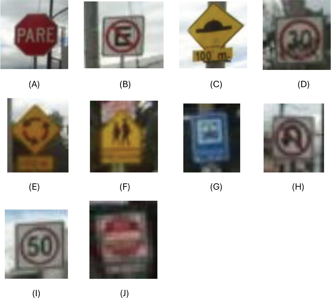
Figure 3:
(A) Ecuadorian stop, (B) no stopping or parking, (C) speed bump ahead, (D) 30 km/h speed limit, (E) roundabout ahead, (F) school zone (G) bus stop, (H) no U-turn, (I) 50 km/h speed limit, (J) no entry.
b. Annotation process
The annotation process involved manually drawing bounding boxes around each traffic sign in all images using Roboflow and exporting the results as a YOLO file, as shown in Figure 4. This process had two stages: initial annotation of all images, followed by a secondary review for reliability. Blurry images were included to simulate real driving conditions and enhance model robustness.
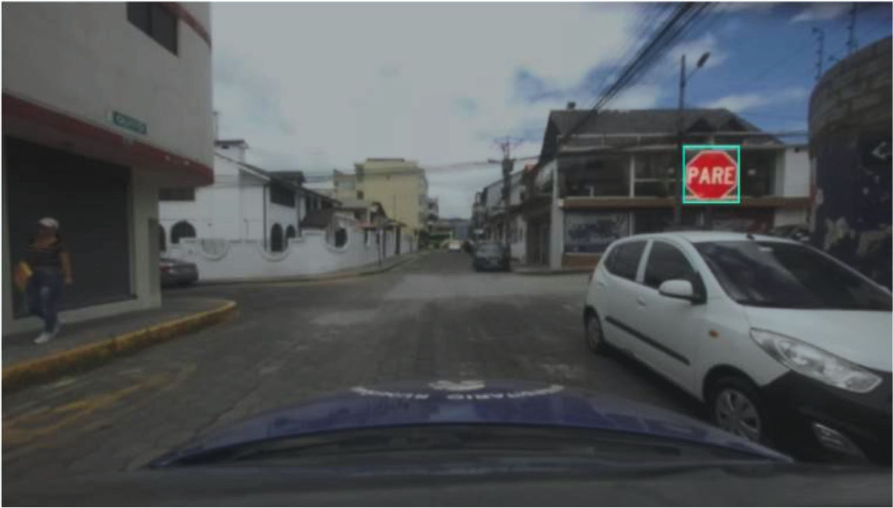
Figure 4:
Image annotation.
c. Model training
The YOLO algorithm focuses on real-time object detection based on a CNN architecture in a direct regression approach. The input images are pre-normalized to a fixed size of 640 × 640 × 3 to ensure uniform processing. While the dataset size is limited compared to large-scale datasets, it is justified by the lack of publicly available regional data and the focus on real-world variability. Table 2 highlights the main characteristics of the YOLO models used in this study, trained with the previously created dataset. The training approach consists of adjusting the YOLO models based on the architectures of each model pre-trained on the COCO dataset [33].
Table 2:
Features of YOLO models
| Features | YOLOv11 [34] | YOLOv12 [35] | YOLOv26 [36] |
|---|---|---|---|
| Architecture | Optimized CNN (C3K2, CSP-like) | Attention-centric (efficient attention, R-ELAN) | Simplified CNN + end-to-end NMS-free |
| Post-processing | Requires traditional NMS | Requires NMS | Native end-to-end without NMS |
| mAP COCO (approx. Variant) | ~51%–52% | ~53%–54% (v1 better in some reports) | ~53%–53.1% (slightly superior to YOLO11 in official benchmarks) |
d. Evaluation metrics
The metrics used to evaluate the models obtained are precision (1), recall (2), F1 score (3), average precision (AP), and mean average precision (mAP). At the same time, the performance of each model was evaluated using a confusion matrix. True positives and true negatives represent correctly classified positive and negative samples, while false positives (FP) and false negatives (FN) represent misclassified positive and negative samples.
e. ROS2 node structure
Figure 5 shows the application environment, which leverages the interoperability of ROS2. It also describes the node structure, where the main node captures raw data from/zed/zed_node/rgb/image_rect_color from the zed 2i depth camera. The images are sent to the traffic/signs_node node, where the YOLO model (YOLOv11, YOLOv12, or YOLOv26) detects and classifies traffic signs. Finally, the traffic/signs_node/class node sends the detected and classified sign class to the output.
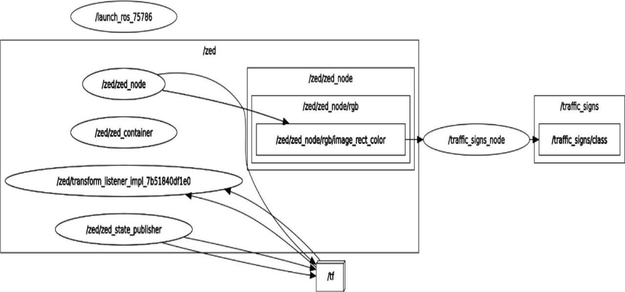
Figure 5:
RQT graph illustrates the communication between the zed 2i camera and the traffic sign detection node.
IV. Results and Discussion
The training parameters and experimental configuration are shown in Tables 3 and 4.
Table 3:
Computing infrastructure for model training
| Name | Type |
|---|---|
| CPU | CPU 4 cores |
| GPU | T4 |
| RAM | 16 GB |
| Framework | PyTorch |
Table 4:
Model training parameters
| YOLOv11 | YOLOv12 | YOLOv26 | |
|---|---|---|---|
| Epochs | 150, 200 | 150, 200 | 150, 200 |
| Batch size | 16 | 16 | 16 |
| Optimal algorithm | Adam | Adam | Adam |
| Model weight | YOLOv11n | YOLOv12n | YOLOv26n |
Table 5 compares the performance of YOLOv11n, YOLOv12n, and YOLOv26n models at epochs 150 and 200. The models were evaluated based on the metrics of precision, recall, mAP@50, and mAP@50–95.
Table 5:
Performance metrics of the YOLOv11n, YOLOv12n, and YOLOv26n models at 150 and 200 epochs
| Models | Epochs | Precision | Recall | mAP50 | mAP50-95 |
|---|---|---|---|---|---|
| YOLOv11n | 150 | 0.69353 | 0.92976 | 0.96008 | 0.65295 |
| YOLOv11n | 200 | 0.69625 | 0.91667 | 0.94615 | 0.65097 |
| YOLOv12n | 150 | 0.70033 | 0.94868 | 0.99386 | 0.66485 |
| YOLOv12n | 200 | 0.9263 | 0.7375 | 0.88789 | 0.63377 |
| YOLOv26n | 150 | 0.8091 | 0.81977 | 0.896 | 0.63967 |
| YOLOv26n | 200 | 0.93036 | 0.63968 | 0.77258 | 0.55697 |
The YOLOv12n model achieves the best performance during the 150 epochs, with an accuracy of 0.70033, recall of 0.94868, mAP@50 of 0.99386, and mAP@50-95 of 0.66485. These scores indicate high accuracy in object detection and localization.
In the YOLOv11n model, better results are achieved in 150 epochs than in 200 epochs. On the other hand, for the YOLOv26n model, an increase in accuracy (0.93036) was achieved during the 200 epochs, but this led to a reduction in recall (0.63968), as well as a decrease in mAP values. These results indicate that the models exhibit an overfitting effect.
For all models, extending training to 200 epochs does not improve performance, and therefore, the 150-epoch configuration provides better performance.
In Figure 6, the YOLOv11 model has a smooth and gradual convergence in all loss components, indicating stable optimization dynamics. Compared to the YOLOv11 model, the YOLOv12 model shows a faster drop in classification, confirming greater efficiency in class prediction learning. On the other hand, the YOLOv26 model exhibits an initial classification loss, indicating aggressive learning. In terms of validation loss analysis, the YOLOv12 model shows the most stable curves compared to the YOLOv11 and YOLOv26 models, suggesting better generalization stability. Under the criteria of detection performance metrics, accuracy, and recall, the YOLOv12 model demonstrates a better balance compared to the YOLOv11 and YOLOv12 models, which show fluctuations between epochs. The convergence of each model was identified when the mAP@0.5 exceeded 0.85. The YOLOv12 model reached this threshold in the first 45 epochs, while the YOLOv11 and YOLOv26 models needed 55 to 60 epochs, meaning that YOLOv12 has faster learning dynamics. YOLOv12 also improves the mAP@0.5 by 3% compared to YOLOv11 and 4% compared to YOLOv26. Overall, the YOLOv12 model confirms superior performance across all metrics. Even though the YOLOv26 model reports competitive detection performance, it also demonstrates greater classification loss and greater validation variability. It is also true that YOLOv11 records consistent results but achieves lower accuracy.
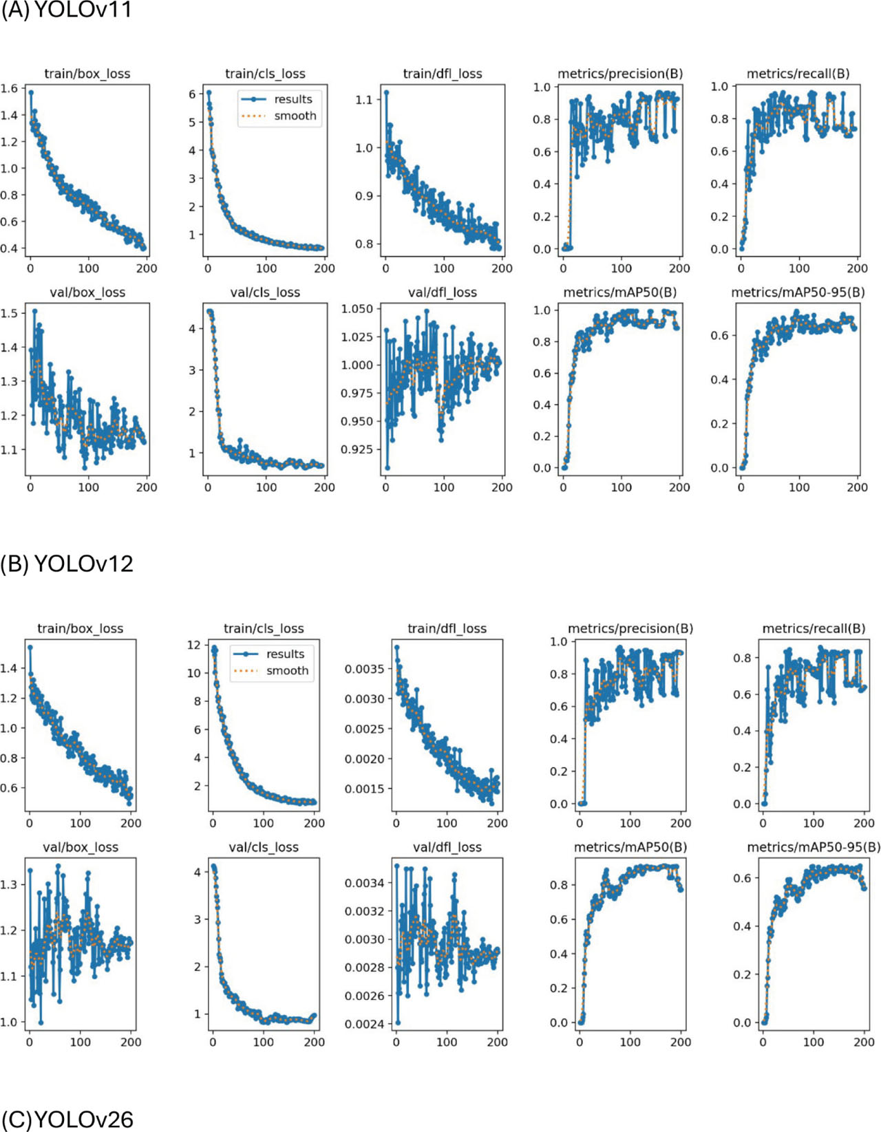
Figure 6:
The training and validation losses of YOLOv11 (A), YOLOv12 (B), and YOLOv26 (C).
Figure 7 shows a comparison of training and validation between YOLOv11 (A), YOLOv12 (B), and YOLOv26 (C) at epochs 150–200. The YOLOv11 and YOLOv12 models show a decrease in training losses in the first 20–40 epochs. After epochs 60–80, the curves are flat, with only small increases. In YOLOv26, there is a sharp drop in classification losses in epochs 50–60. All models show that most learning occurs in the early epoch and then with diminishing returns.
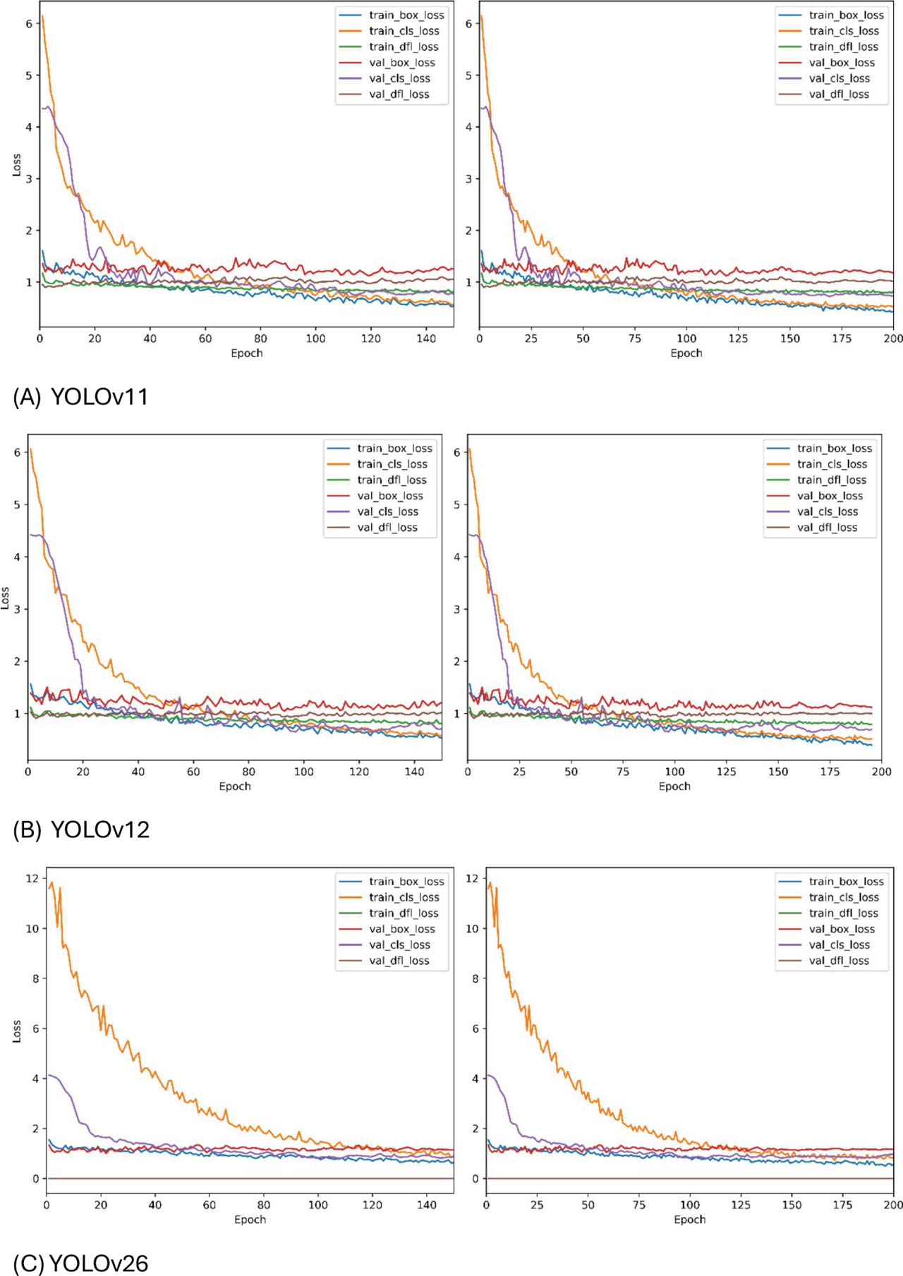
Figure 7:
Comparative analysis between the 150 and 200 epochs of YOLOv11 (A), YOLOv12 (B), and YOLOv26 (C).
Figure 8 shows a comparison of the YOLOv11 (A), YOLOv12 (B), and YOLOv26 (C) models in epochs 150–200 in mAP@50 and mAP@50. In the initial epochs, all three models increase significantly, then stabilize and converge. The YOLOv12 model improves mAP@50 by 1%–2% compared to YOLOv11. On the other hand, there is a similar statistical performance between YOLOv12 (B) and YOLOv26 (C). The mAP@50-95 value is below mAP@50 by 0.25%–0.30%, reflecting that the models lose slightly in accuracy in the matching criterion.
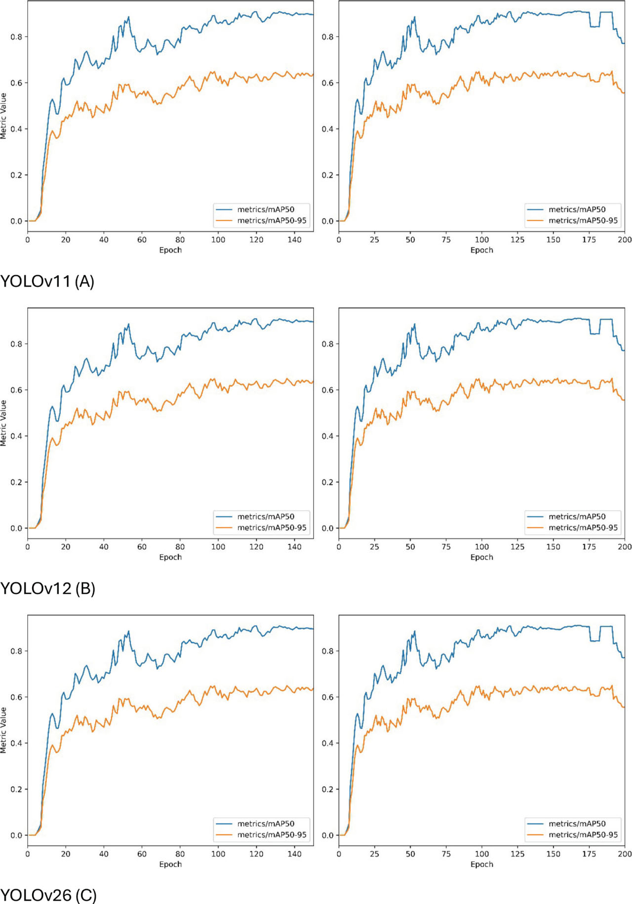
Figure 8:
Smoothed metrics for mAP@50 and mAP@50-95 over 150 epochs and 200 epochs of YOLOv11 (A), YOLOv12 (B), and YOLOv26 (C).
The hyperparameter settings were modified as shown in Table 6.
Table 6:
Changed training parameters of the YOLO models
| Parameter | Value |
|---|---|
| epochs | 200 |
| imgz | 640 |
| batch | 64 |
| lr0 | 0.01 |
| warmup_epochs | 3.0 |
| warmup_bias_lr | 0.1 |
| momentum | 0.8 |
| weight_decay | 0.0005 |
| optimizar | SGD |
| amp | True |
The results of the YOLOv11 (A), YOLOv12 (B), and YOLOv26 (C) models are shown in Table 7. The YOLOv12 model continues to show better performance, achieving high values for mAP50 (0.9625) and mAP50-95 (0.6530) as well as recall (0.7573), resulting in better detection and localization capabilities compared to the YOLOv11 (A) and YOLOv26 (C) models.
Table 7:
Performance metrics with changes to the YOLOv11n, YOLOv12n, and YOLOv26n models over 200 epochs
| Models | Epochs | Precision | Recall | mAP50 | mAP50-95 |
|---|---|---|---|---|---|
| YOLOv11n | 200 | 0.95611 | 0.72357 | 0.87374 | 0.60009 |
| YOLOv12n | 200 | 0.92965 | 0.75729 | 0.96251 | 0.65297 |
| YOLOv26n | 200 | 0.93036 | 0.63968 | 0.77258 | 0.55697 |
Figure 9 shows that the YOLOv12 (B) model has a faster and more stable convergence, with lower validation losses. This clarifies that this model continues to offer the best balance between convergence, accuracy, and performance compared to the other three models. On the other hand, the YOLOv26 (C) model continues to show fluctuations in validation losses and relatively low final metrics, indicating less stable performance. Finally, the YOLOv11 (A) model shows moderate fluctuations in validation losses.
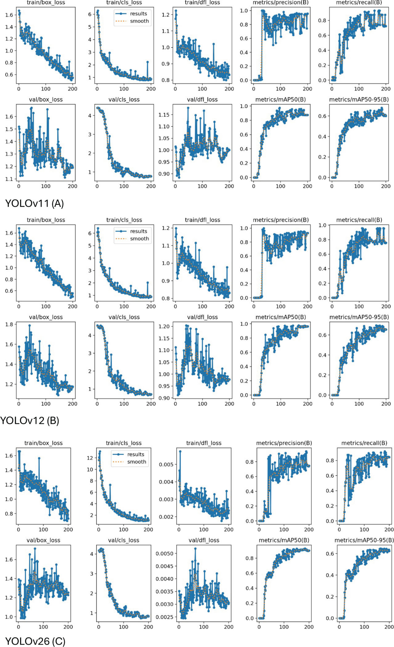
Figure 9:
The training and validation losses of YOLOv11 (A), YOLOv12 (B), and YOLOv26 (C) after the parameter change.
Figure 10 shows the detection of different traffic signs in YOLOv11 (A), YOLOv12 (B), and YOLOv26 (C) models in different environmental conditions. The identification of each category is also shown along with the confidence score in each image. The performance of each model can also be analyzed in detail. Both YOLOv11 (A) and YOLOv26 (C) show excellent performance in traffic sign detection, with YOLOv12 (B) being the most accurate. It is also worth mentioning that each model highlights different capabilities in identifying characteristics related to traffic signs.
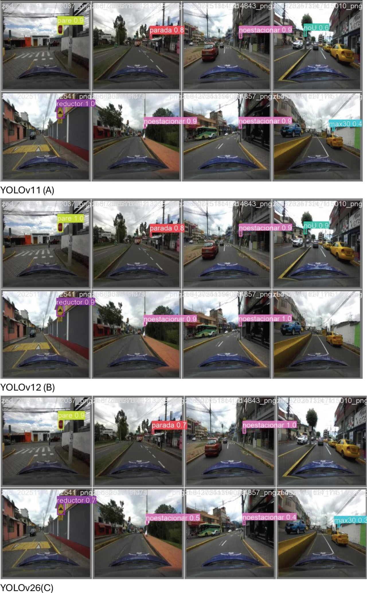
Figure 10:
Examples of traffic sign detections of YOLOv11 (A), YOLOv12 (B), and YOLOv26 (C).
There are instances where the models do not correctly detect or classify traffic signs, as shown in Figure 11. In the case of FN: (A) and (B), the model does not detect any traffic signs. For FP: (B) and (C), there is incorrect detection and labeling.
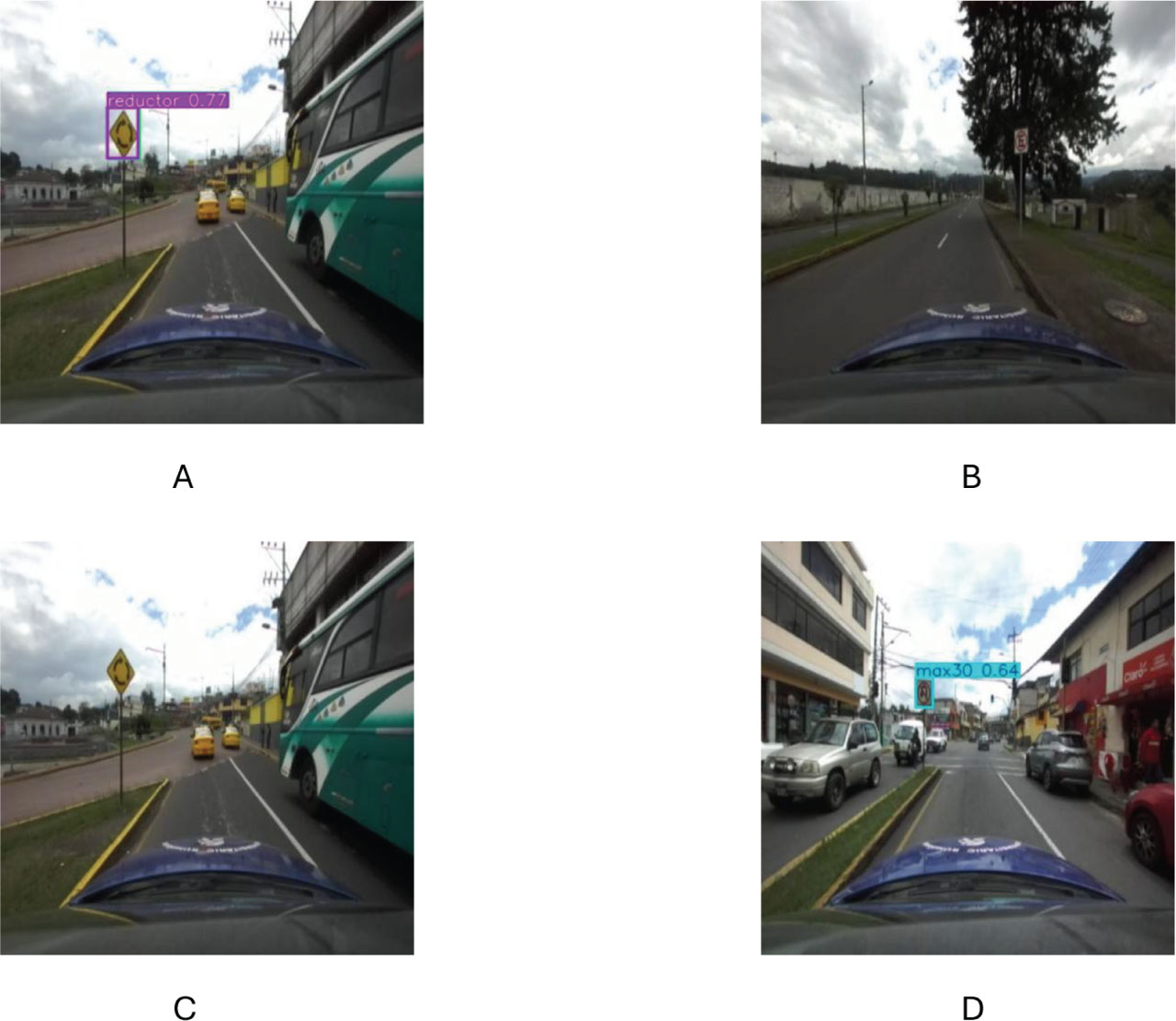
Figure 11:
Examples of FP (A,D) and FN (B,C). FN, false negatives; FP, false positives.
The results demonstrate that YOLOv12 consistently outperforms YOLOv11 and YOLOv26 in terms of mAP, recall, and convergence speed. Compared to previous studies in Ecuador that rely on CNN or R-CNN models [3, 7, 29, 30,31,32], the evaluated YOLO architectures show superior real-time performance and detection accuracy. These findings align with recent literature highlighting the efficiency of YOLO-based detectors. The superior performance of YOLOv12 is attributed to its attention-based architecture. Also, overfitting at higher epochs indicates that smaller datasets require careful training control.
A key strength of this study is the use of real-world Ecuadorian data and ROS2 integration. However, limitations include a relatively small dataset size and a restriction to 10 traffic sign classes.
V. Conclusions and Future Work
This study evaluated the performance of YOLO models (YOLOv11, YOLOv12, YOLOv26) for traffic sign detection in Ecuadorian urban environments. The YOLOv12 model stands out with the best metrics: precision (0.70033), recall (0.94868), mAP@50 (0.99386), and mAP@50-95 (0.66485).
Under the initial configuration, the YOLOv12 model provided the highest mAP50 (0.99386) and the highest recall (0.94868) in the first 150 epochs. Increasing the number of epochs in training did not improve performance, suggesting that overfitting may occur when trained for longer periods. In the second configuration, all models showed higher precision but lower recall, which generates fewer FP but omits more objects. The comparative analysis in this study also showed that each model’s performance is strongly related to both the architecture and the configuration of the hyperparameters.
In future work, the authors will use an experimental design to compare the estimated distance by bounding box with the actual depth. Further, a calculation of the time remaining to reach the traffic signal will be included to contribute to the development of advanced driver assistance applications. Also, future work includes expanding the dataset.
Abbrevations
- 3D:
Three-Dimensional;
- AP:
Average Precision;
- AUC:
Area Under the Curve;
- COCO:
Common Objects in Context;
- CPU:
Central Processing Unit;
- GPU:
Graphics Processing Unit;
- GTSDB:
German Traffic Sign Detection Benchmark;
- GTSRB:
German Traffic Sign Recognition Benchmark;
- HOG:
Histogram of Oriented Gradients;
- LISA:
Laboratory for Intelligent and Safe Automobiles;
- LTS:
Long Term Support;
- mAP50:
Mean Average Precision at an Intersection over Union (IoU) threshold of 0.50;
- mAP50-95:
Mean Average Precision averaged over Intersection over Union (IoU) thresholds ranging from 0.50 to 0.95;
- RAM:
Random Access Memory;
- R-CNN:
Region-Based Convolutional Neural Network;
- R-ELAN:
Residual Efficient Layer Aggregation Networks;
- RGB:
Red-Green-Blue;
- ROS:
Robot Operating System;
- RQT:
ROS Qt-based Graphical User Interface Framework;
- RTK:
Real-Time Kinematic;
- SGD:
Stochastic Gradient Descent;
- TT100K:
Tsinghua-Tencent 100K Traffic Sign Dataset;
- YOLO:
You Only Look Once;
- YOLOv11:
You Only Look Once Version 11;
- YOLOv12:
You Only Look Once Version 12;
- YOLOv26:
You Only Look Once Version 26;
- ZED:
Stereo camera developed by Stereolabs;
- ZED-2i:
Stereolabs ZED 2i stereo camera;
- ZF-Net:
Zeiler and Fergus Network.
Notes
Acknowledgment
The authors would like to thank Instituto Superior Tecnológico Rumiñahui, located in Sangolquí, Ecuador, for its support in the development of this research.