
Table 1:
Comparative analysis of existing works
| References | Techniques | Advantages | Disadvantages |
|---|---|---|---|
| Mou et al. [21] | SCSO algorithm | High gain, fast convergence | Complex parameter tuning |
| Liu et al. [22] | CTPOA | High efficiency | Complex structure |
| Li et al. [23] | DO algorithm | Fast convergence | High complexity, parameter sensitivity |
| Raghuvanshi et al. [24] | MAOA | Low SLL, balanced optimization | Complex design, slower execution |
| Cheng et al. [25] | APSO | Fast convergence, high robustness | Complex tuning, high computation |
| Manai et al. [26] | modified RD-MUSIC | Reduced interference, high SINR, low complexity | High processing demand, sensitive to DoA |
[i] APSO, adaptive particle swarm optimization; CTPOA, chaos triangular pelican optimization algorithm; DO, Dandelion optimization; DoA, direction of arrival; MAOA, modified arithmetic optimization algorithm; MUSIC, multiple signal classification; SCSO, Sand Cat Swarm Optimization; SINR, signal to interference plus noise ratio; SLL, sidelobe level.
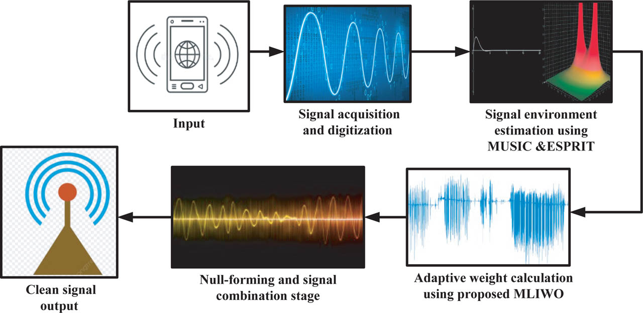
Figure 1:
Block diagram for the proposed methodology. MUSIC, multiple signal classification; ESPRIT, estimation of signal parameters via rotational invariance techniques.
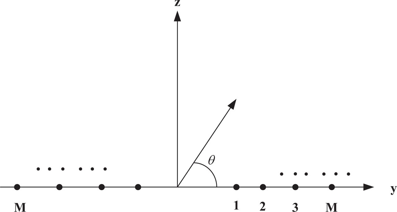
Figure 2:
Geometry of the linear 2N-element symmetrically placed antenna array.
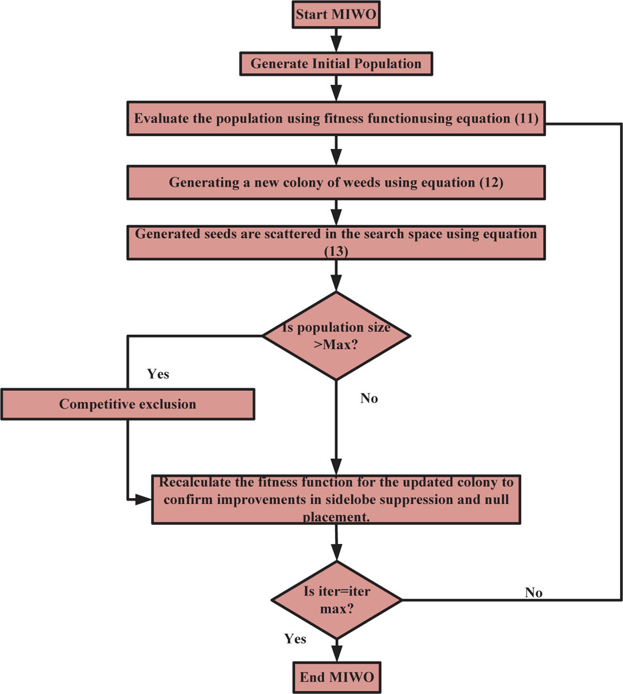
Figure 3:
Flowchart for MIWO algorithm.
Table 2:
Parameter specifications
| Parameter | Value | |
|---|---|---|
| 1 | Maximum number of seeds | 5 |
| 2 | Minimum number of seeds | 0 |
| 3 | Initial standard deviation | 0.1 |
| 4 | Final standard deviation | 0.00015 |
| 5 | Maximum population size | 20 |
| 6 | Number of iterations for local search | 3 |
| 7 | Initial population size | 10 |
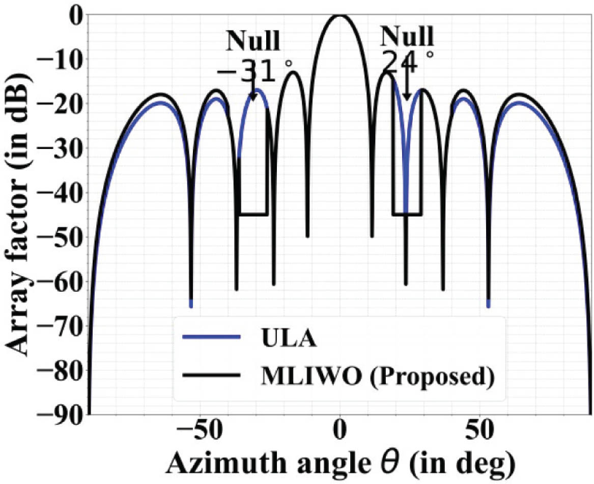
Figure 4:
Radiation pattern analysis of a 10-element linear array with nulls at 24° and −31°. ULAs, uniform linear arrays.
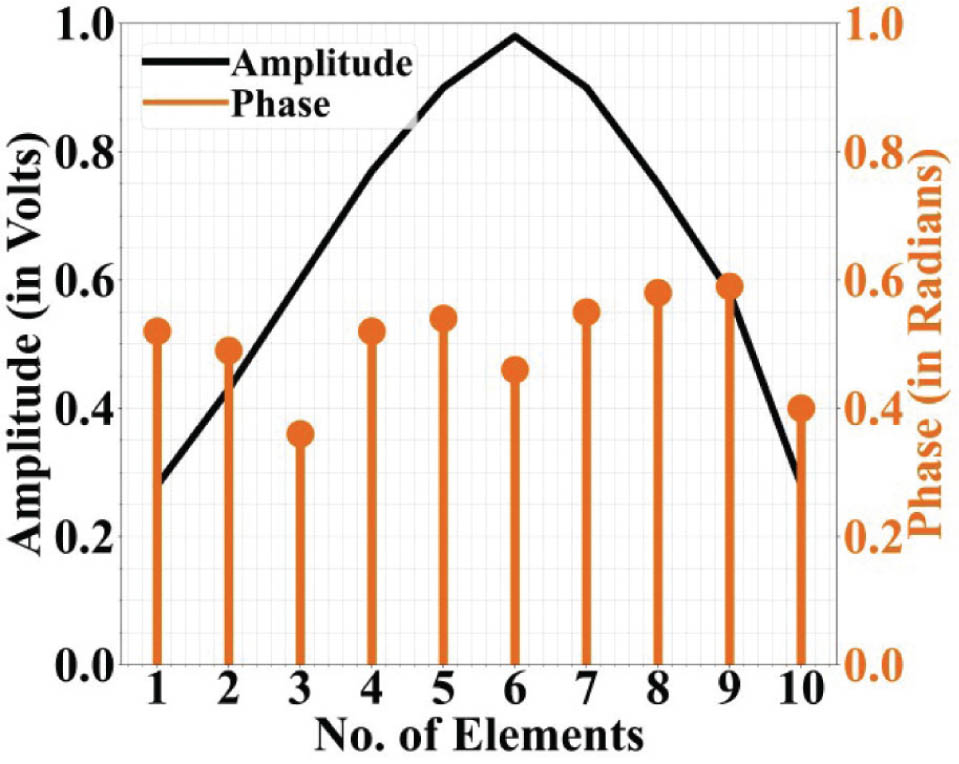
Figure 5:
Optimized phase values and Taylor amplitude distribution for a 10-element linear array with nulls at 24° and −31°.
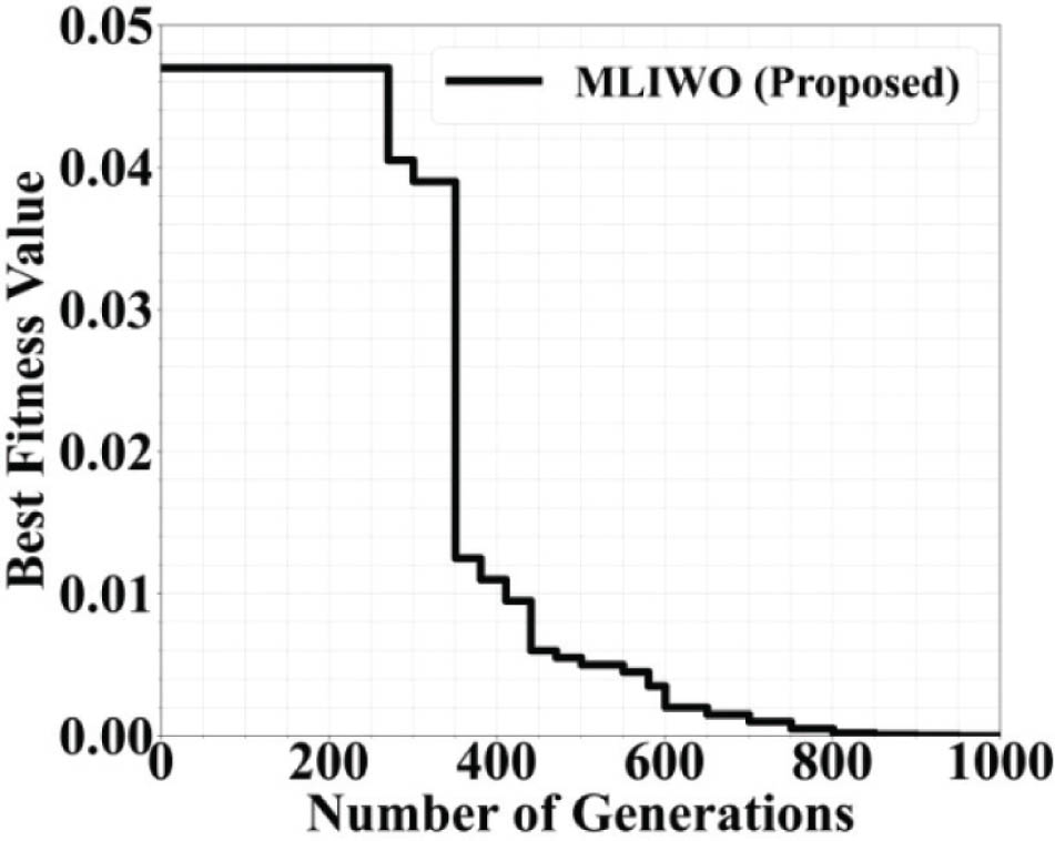
Figure 6:
Convergence plot for a 10-element linear array using MLIWO.
Table 3:
Runtime and convergence comparison of optimization algorithms (10-element array)
| Algorithm | Runtime (s) | Iterations to convergence | Best fitness value | Improvement over GA (%) |
|---|---|---|---|---|
| MLIWO | 12.48 | 520 | 0.0023 | +35.7 |
| IWO | 15.93 | 680 | 0.0042 | +18.6 |
| PSO | 17.81 | 720 | 0.0051 | +10.5 |
| CSO | 18.12 | 740 | 0.0048 | +12.2 |
| GA | 20.32 | 800 | 0.0063 | Baseline |
Table 4:
Comparison of the synthesized results of a 10-element linear array
| Parameter | MLIWO | IWO | CSO | PSO | GA |
|---|---|---|---|---|---|
| PSLL (in dB) | −24.01 | −21.05 | −20.83 | −19.85 | −18.10 |
| Null at 31° (in dB) | −78.92 | −75.25 | −69.56 | −70.11 | −65.84 |
| Null at −45° (in dB) | −70.59 | −65.17 | −68.54 | −65.89 | −62.85 |
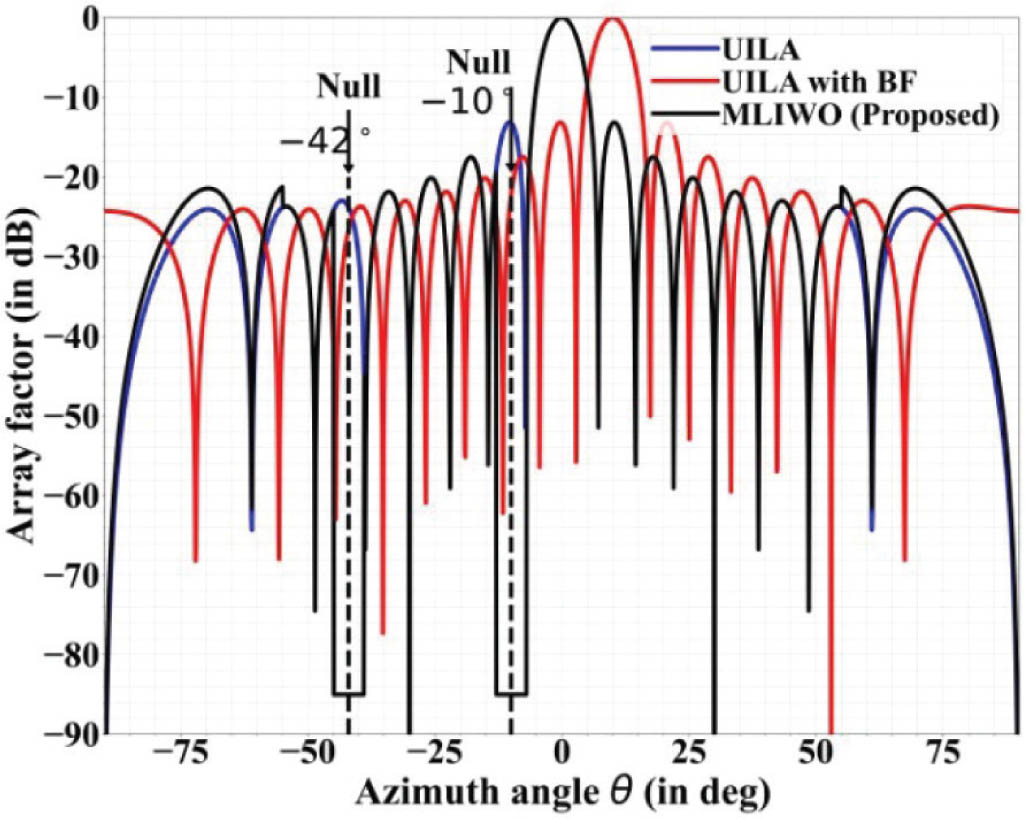
Figure 7:
Radiation pattern of a 20-element linear array with 23° beam steering, and nulls at −10° and −42°. UILA, uniform isotropic linear array; BF, Bayesian filtering.
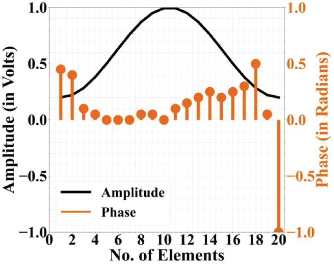
Figure 8:
Optimization of phase and Taylor amplitude distribution for a 20 element linear array with 23° beam steering and nulls at −10° and −42°.
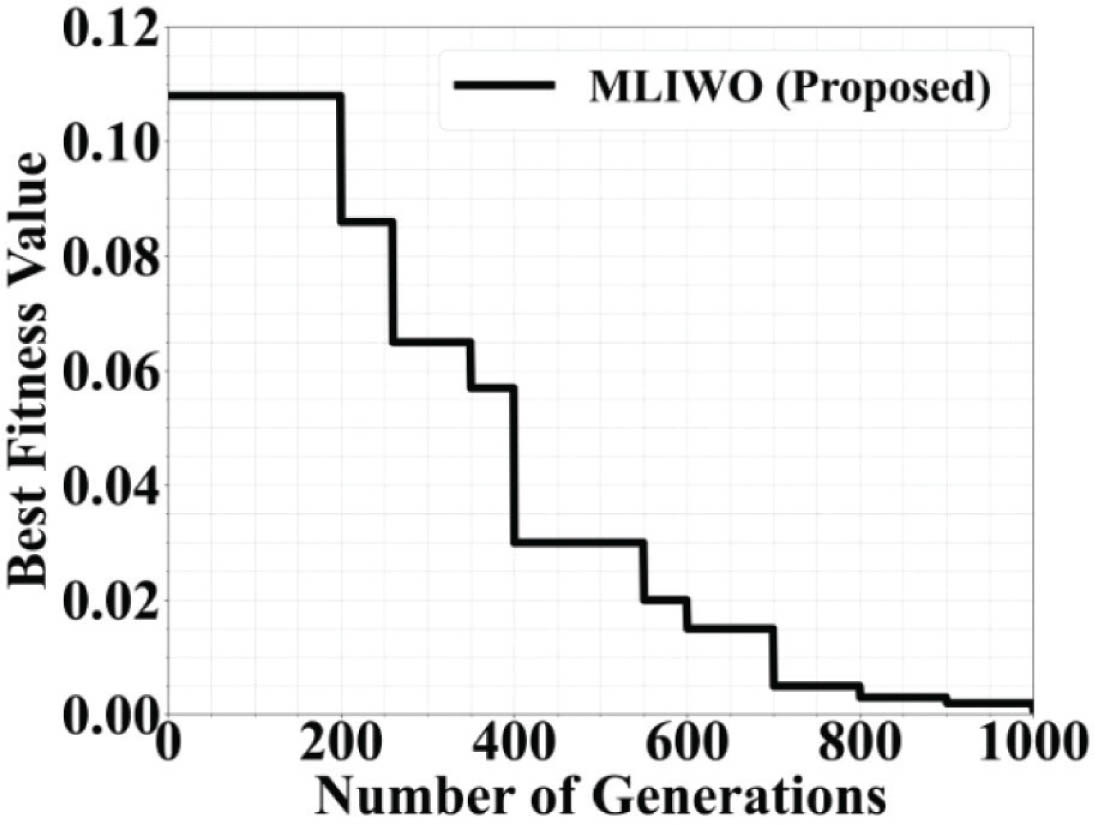
Figure 9:
Convergence plot for a 20-element linear array using MLIWO.
Table 5:
Comparison of synthesized results of a 20 element linear array
| Parameter | MLIWO | IWO | CSO | PSO | GA |
|---|---|---|---|---|---|
| Beam steering (in Deg) | 23° | 23° | 23° | 23° | 23° |
| PSLL (in dB) | −21.80 | −19.41 | −19.82 | −18.20 | −17.52 |
| Null at −10° (in dB) | −80.75 | −71.41 | −72.84 | −69.58 | −61.47 |
| Null at −42° (in dB) | −88.87 | −74.58 | −69.74 | −65.24 | −62.32 |
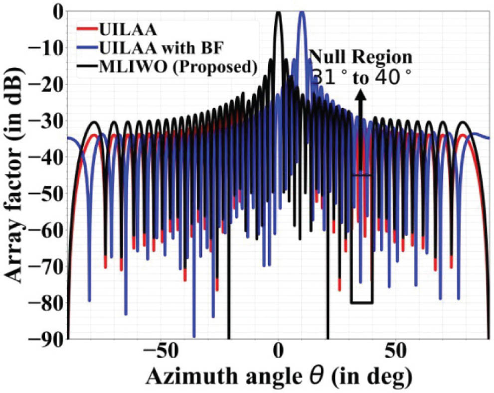
Figure 10:
Radiation pattern analysis of a 100 element linear array with −41° beam steering, and sector null in the angular region of 31° and 40°. UILA, uniform isotropic linear array; BF, Bayesian filtering.
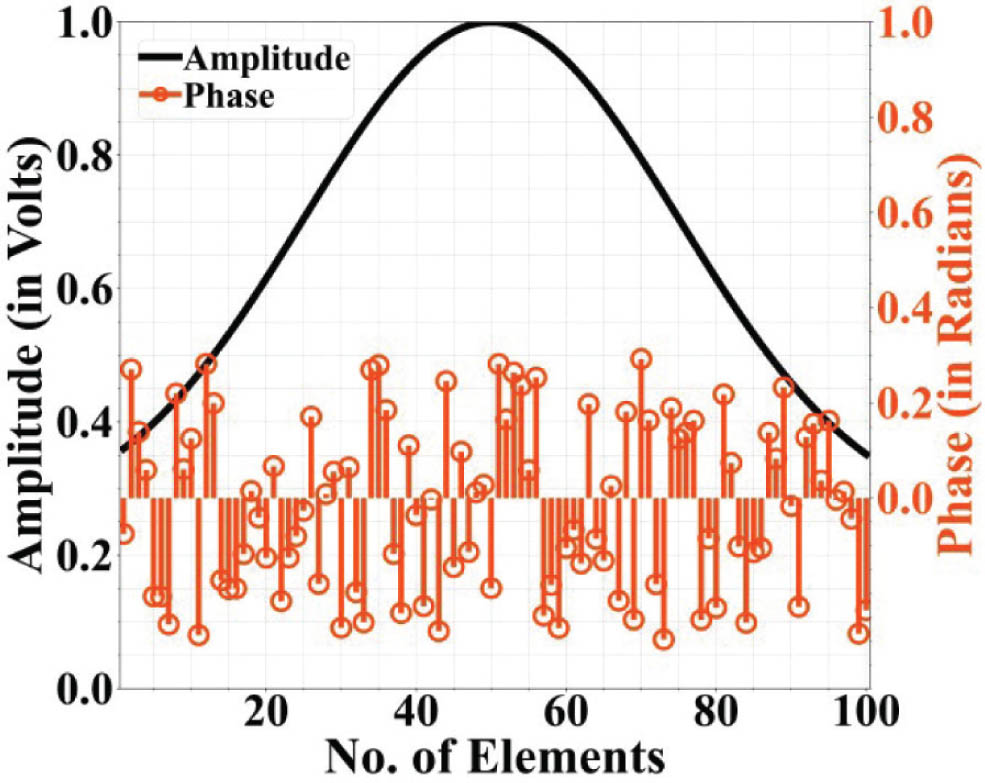
Figure 11:
Phase and amplitude optimization of a 100-element linear array with −41° beam steering, and sector null in the angular region of 31° and 40°.
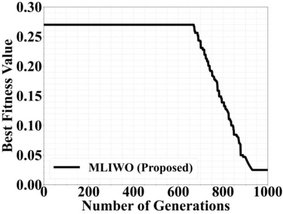
Figure 12:
Convergence plot for a 100-element linear array using MLIWO.