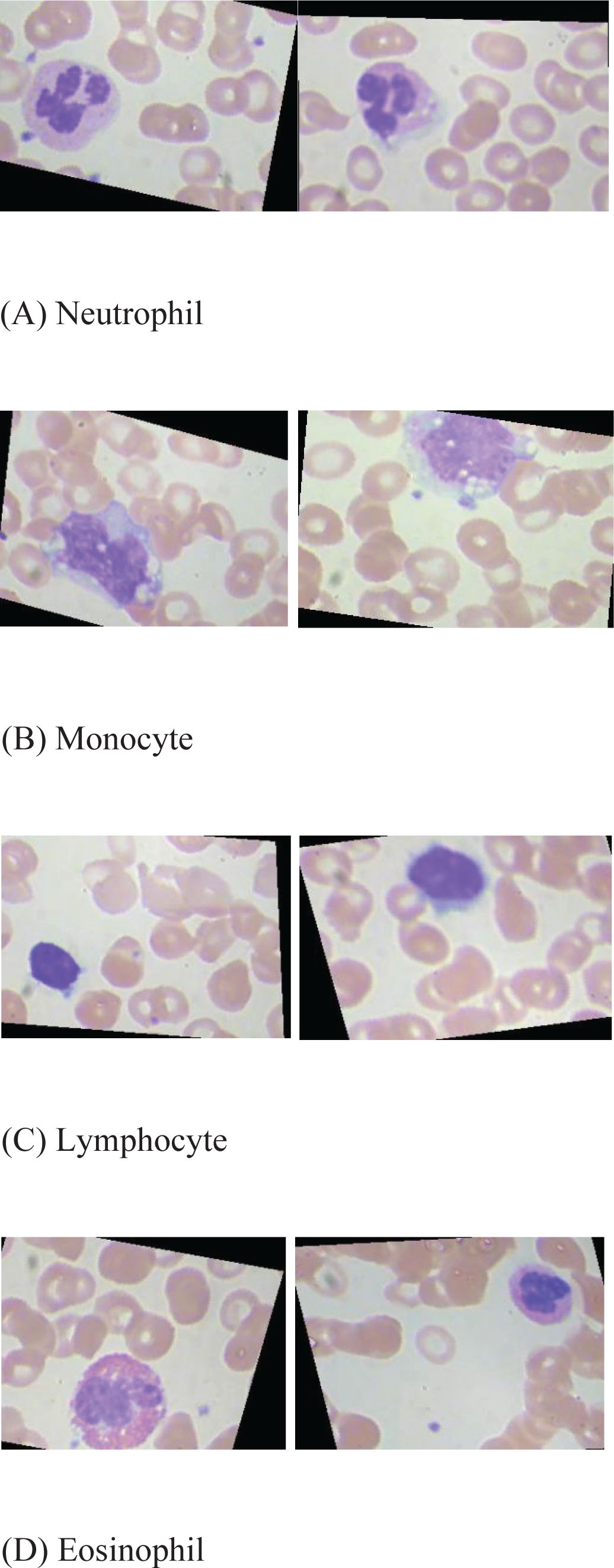
Table 1:
Summary of significant paper for last decade
| Year | Paper ref | Data set | Deep learning models | Accuracy (%) |
|---|---|---|---|---|
| 2016 | [12] | All four classifiers are trained with dataset of 500 instances. | ANN, DT, k-NN, and NB | 96.63 |
| 2023 | [13] | The datasets were collected from10 health facilities across the country | A machine learning approach was used to detect iron-deficiency anemia with the application of NB, CNN, SVM, k-NN, and DT algorithms | 99.12 |
| 2023 | [16] | The suggested technique makes use of time-domain analysis to determine the relationship between blood hemoglobin concentration and palm color variations brought on by applying and releasing pressure. | Dual-mode information fusion with pre-trained CNN models and transformer | 96.29 |
| Processed and analyzed is a smartphone camera sensor that captures the entire event of palm color changes produced by a bespoke gadget. | ||||
| 2023 | [11] | A specially constructed dataset of 2,592 pediatric palpebral images was used in the investigation | UCE, UNet+ +, FCN, PSPNet, and Link Net. | 94.14 |
| 2023 | [15] | After beginning with 527 datasets, the experiment added 2,635 more by utilizing translation, flipping, and rotation. | CNN, k-NN, Naive Bayes’, SVM, and DT were used to build the suggested models for the identification of anemia. | 99.92 |
| 2024 | [14] | The proposed study used a larger size of dataset of 527 conjunctiva images and was then augmented to 2,635 | Machine learning algorithms such as CNN, k-NN, NB, DT, and SVM were utilized for the study to detect anemia | 98.45 |
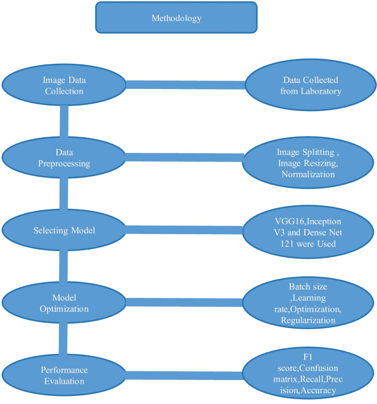
Figure 1:
Methodology.
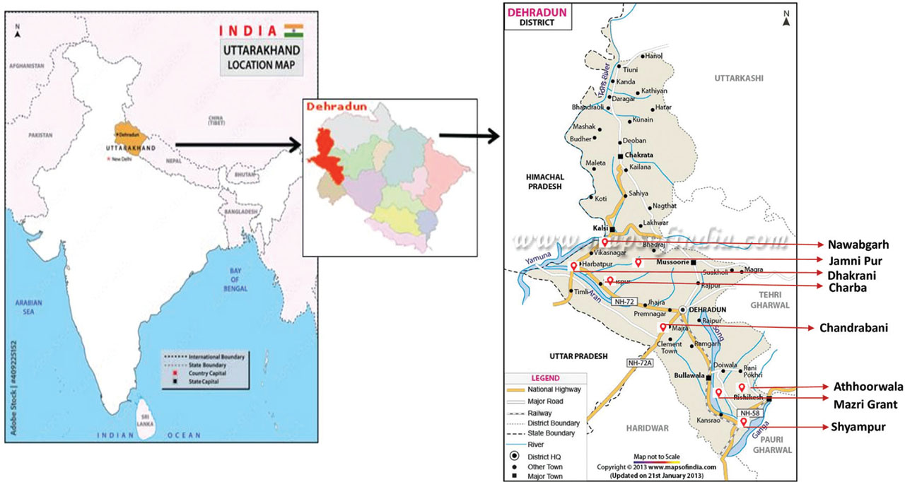
Figure 2:
Site location in Dehradun district.
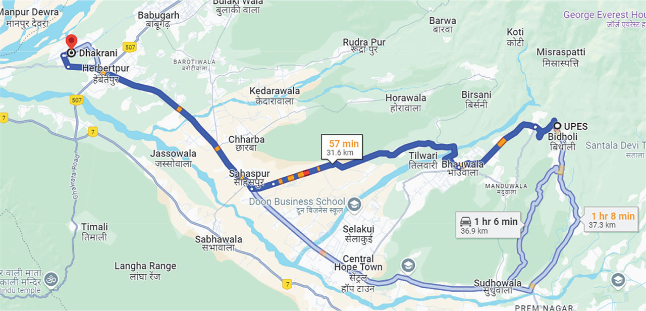
Figure 3:
UPES to Dakrani.
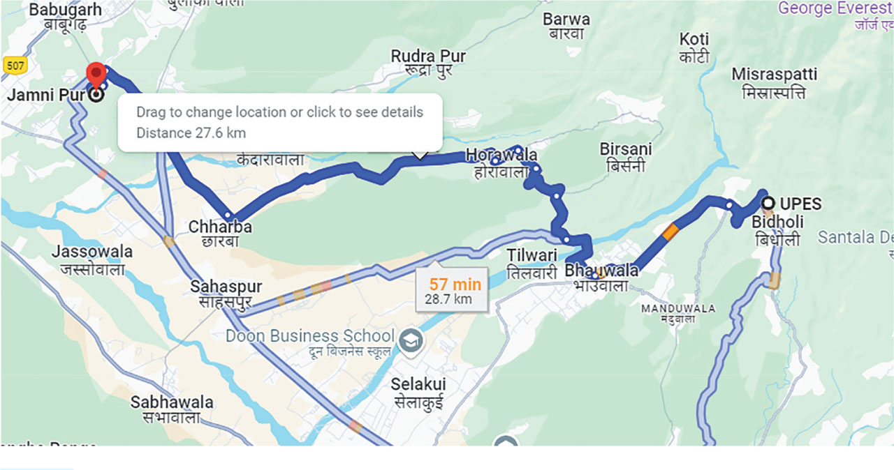
Figure 4:
UPES to Jamnipur.
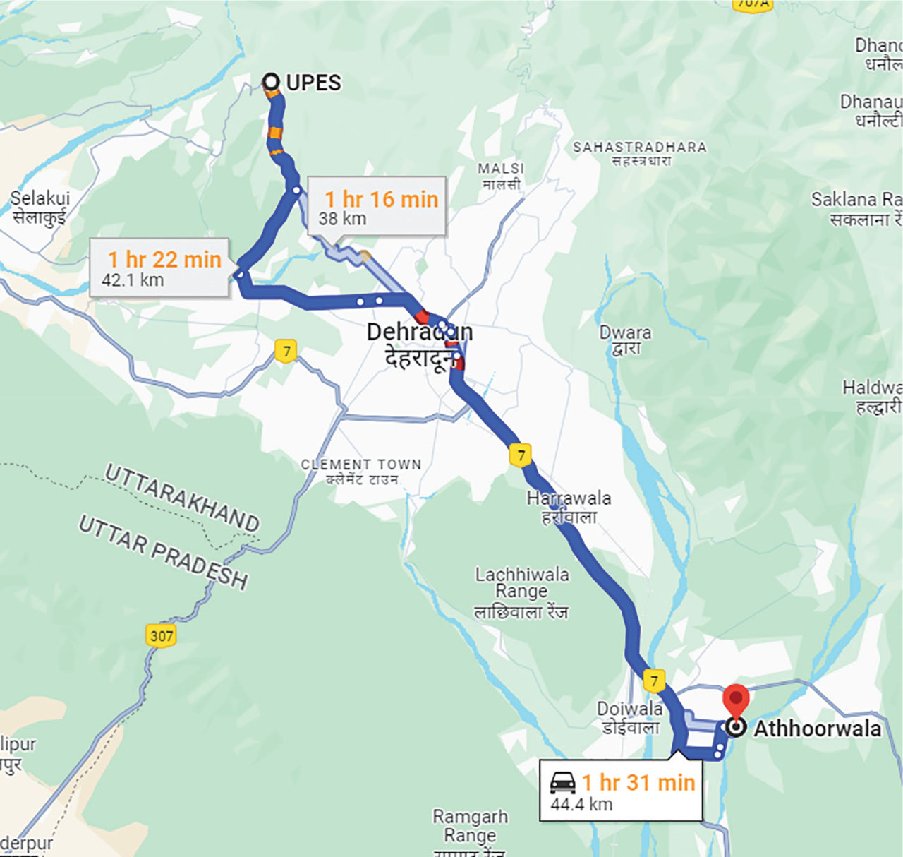
Figure 5:
UPES to Atthorwala.
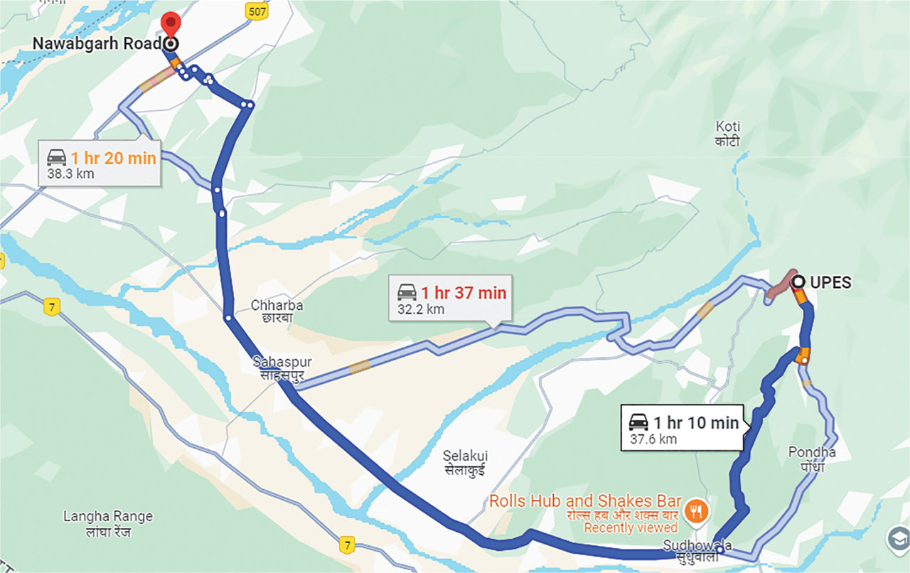
Figure 6:
UPES to Nawabgarh.
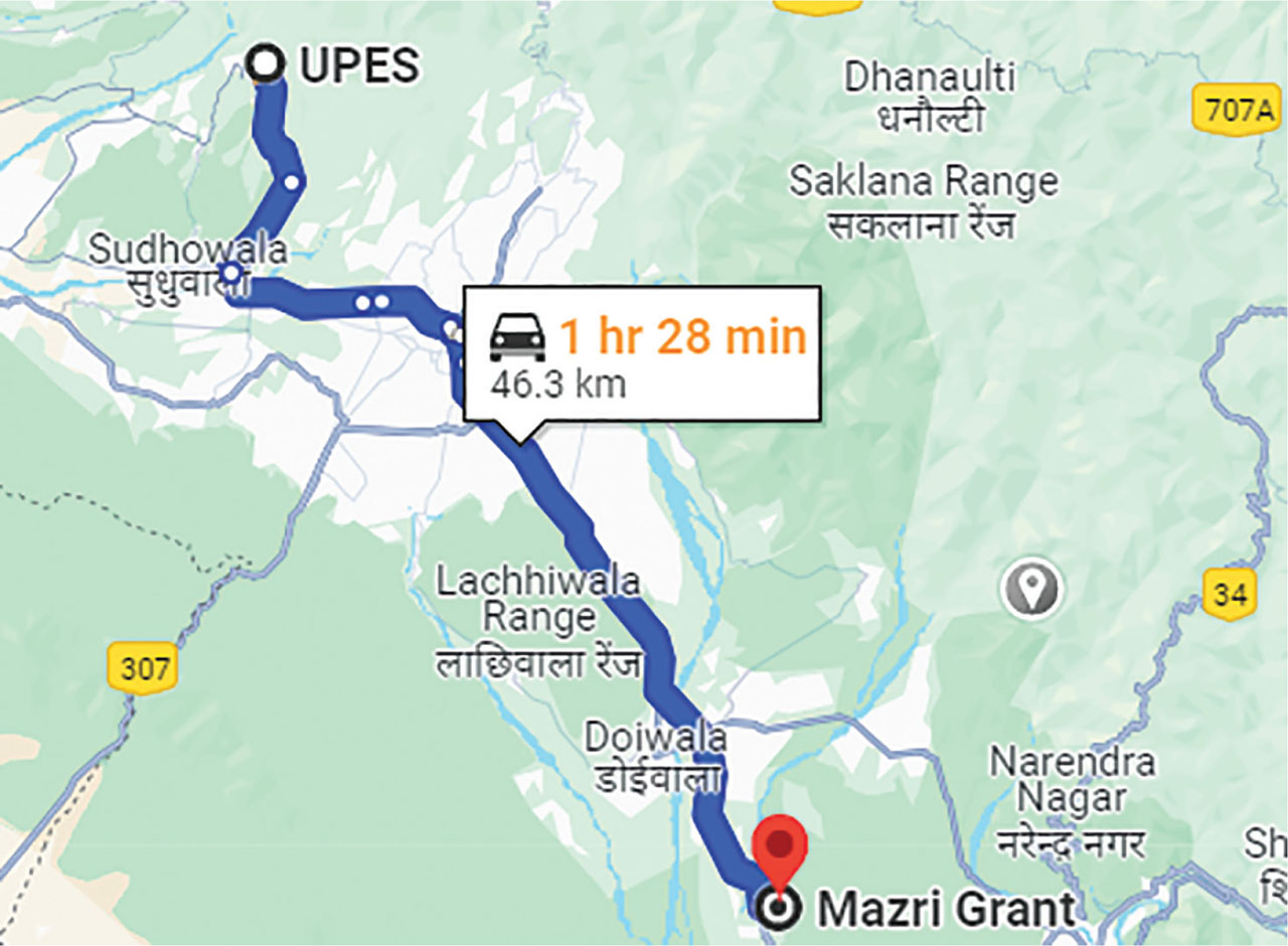
Figure 7:
UPES to Mazri Grant.
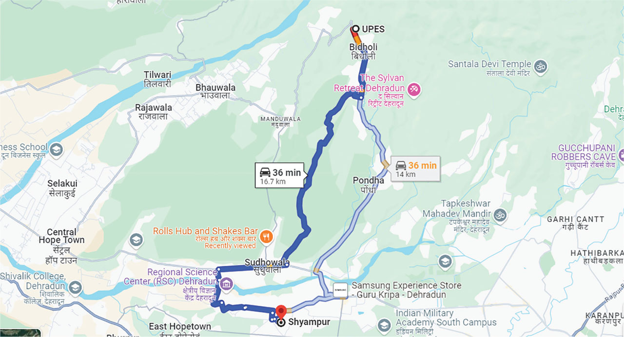
Figure 8:
UPES to Shyampur.
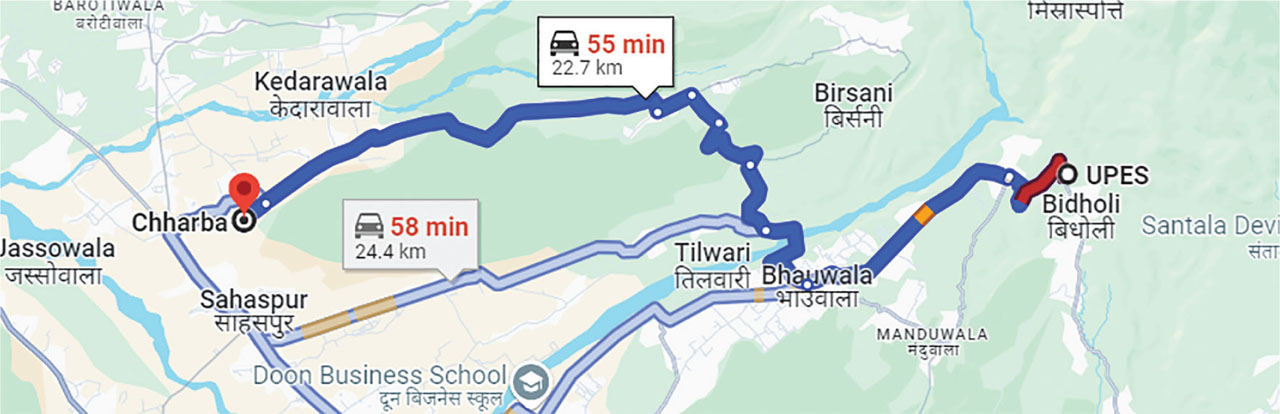
Figure 9:
UPES to Charba.
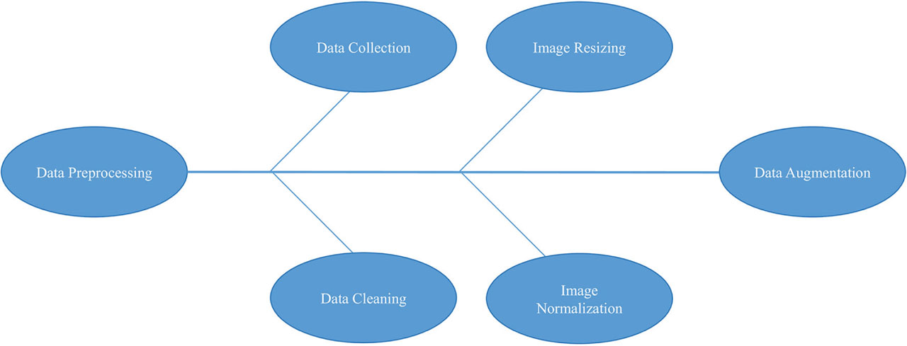
Figure 10:
Data preprocessing.
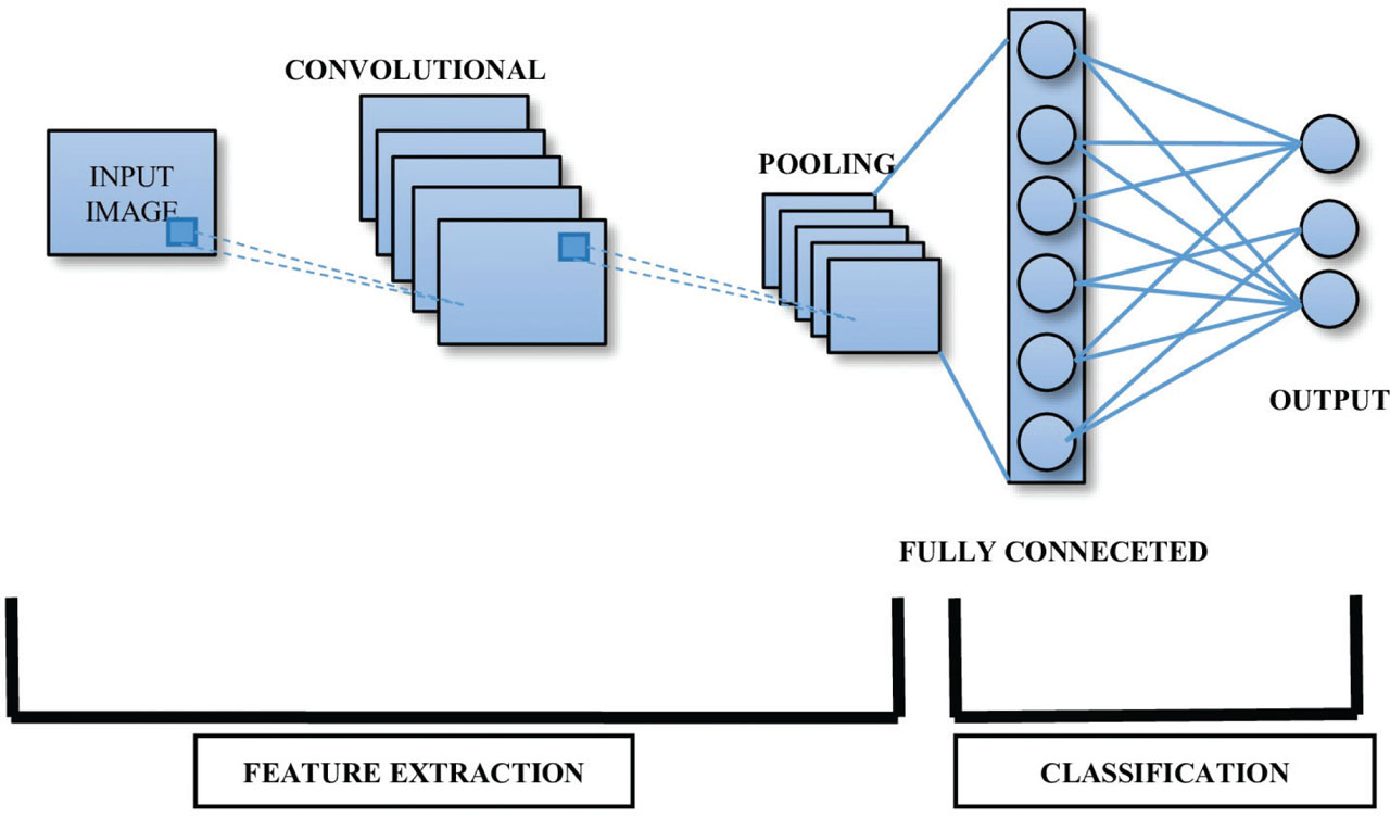
Figure 11:
CNN architecture. CNN, convolutional neural network.
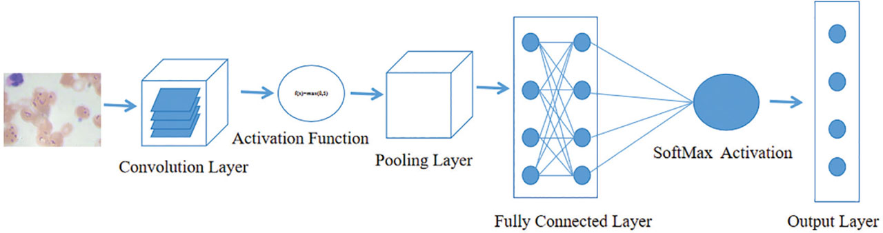
Figure 12:
VGG16 architecture.
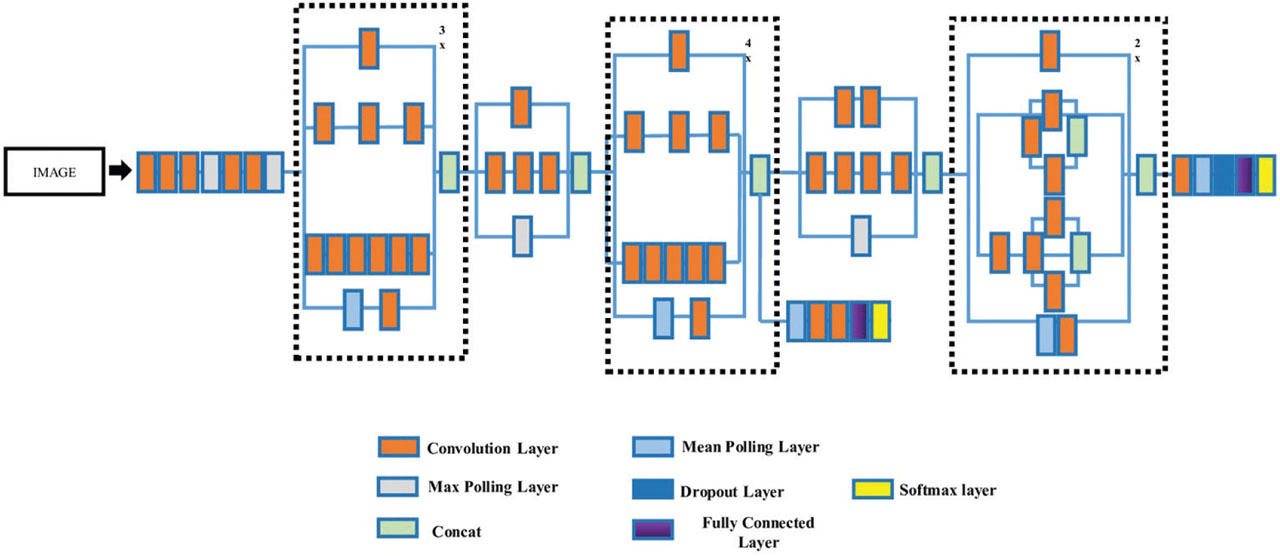
Figure 13:
Inception V3 architecture.
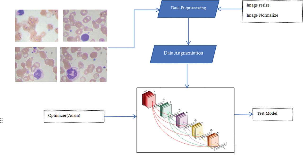
Figure 14:
Applied framework.
Table 2:
About blood cells
| Cell category | Size | Blood life span | Quantity of cells | Functions |
|---|---|---|---|---|
| RBC | 6–8 | 120 days | Male:—4.5–6.5 × 10⁶ | Conveyance of O2 and CO2 |
| Female 3.9–5.6 × 10⁶ | ||||
| Thrombocytes | 0.5–3.0 | 10 days | 140–1,400 × 103 | Coagulation |
| Phagocytes | ||||
| Neutrophils | 12–15 | 6–10 hr | 1.9–7.6 × 10³ (48%–76%) | Protection against microorganisms such as fungi and bacteria |
| Monocytes | 12–20 | 20–40 hr | 0.2–0.8 × 10³ (2.5%–8.5%) | Defense against pathogens like fungi and bacteria |
| Acidophils | 12–15 | Days | 0.04–0.44 × 013 (<5%) | Defence from pathogens |
| Lymphocyte | 7–9 (resting) | Weeks or years | 1.5–3.5 × 10³ (18%–41%) | B-cells: Assist in antibody production and the activation of T-cells. |
| 12–20 (active) | T-cells: Involved in viral defense and immune response | |||
Table 3:
Compare accuracy and time for each epoch based on three deep learning models
| Number of epochs | Accuracy (%) | Batch size | Time for each epoch (in ms) | |
|---|---|---|---|---|
| VGG16 | 90 | 93.43 | 32 | 78 ms/step |
| DenseNet | 90 | 90.48 | 32 | 89 ms/step |
| InceptionV3 | 90 | 78.80 | 32 | 100 ms/step |
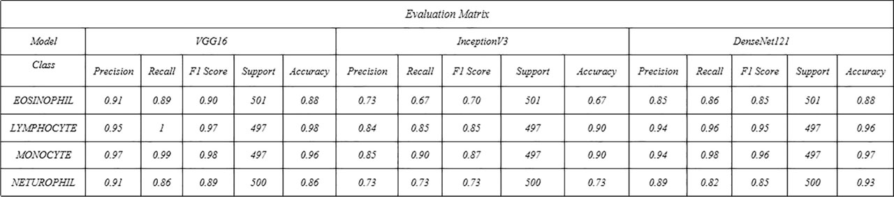
Figure 15:
Evaluation metrics for deep learning models.
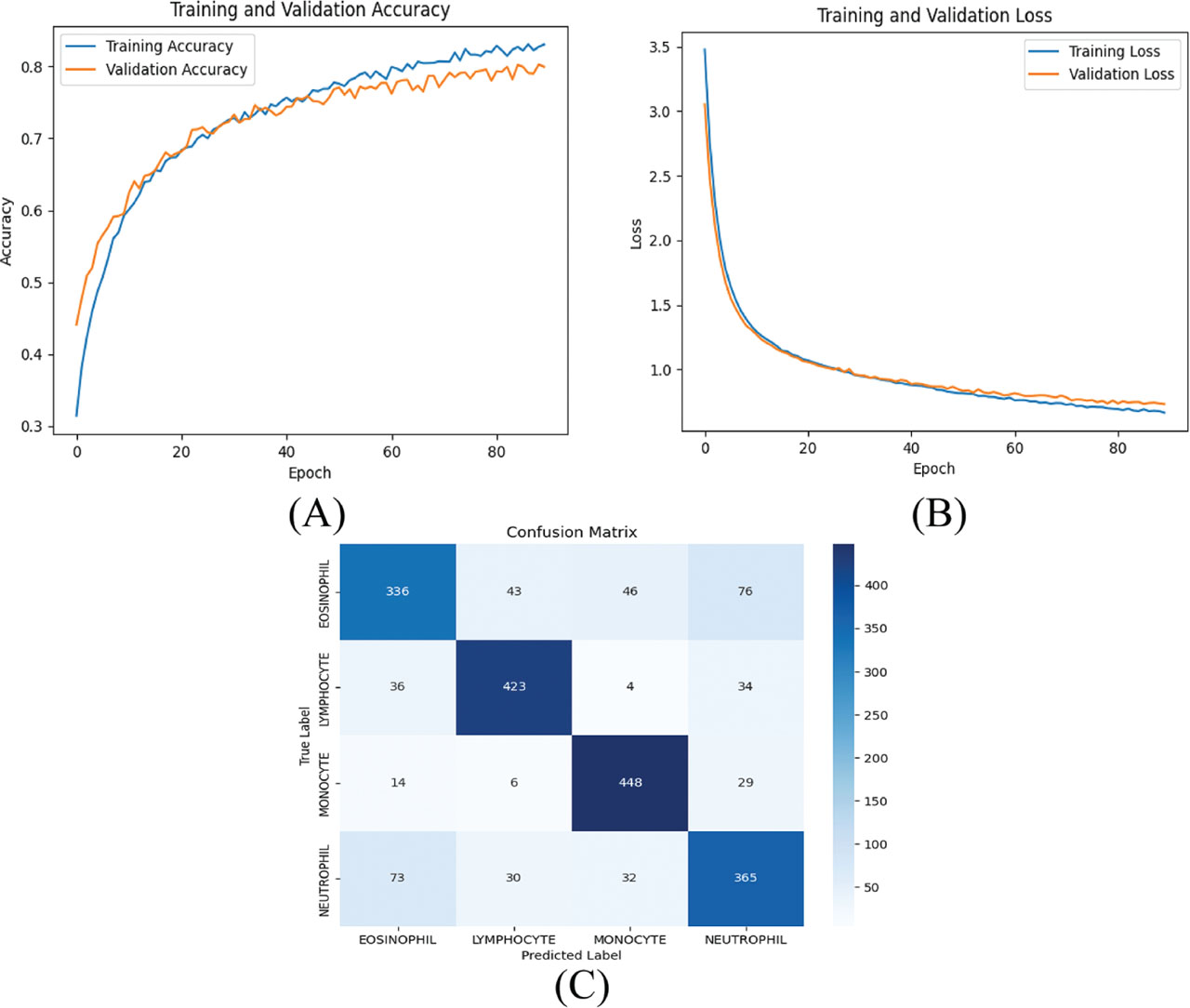
Figure 16:
(A) presents the training and validation accuracy for each epoch, (B) shows the training and validation loss for each epoch, and (C) provides the confusion matrix for each class in the InceptionV3 Model.
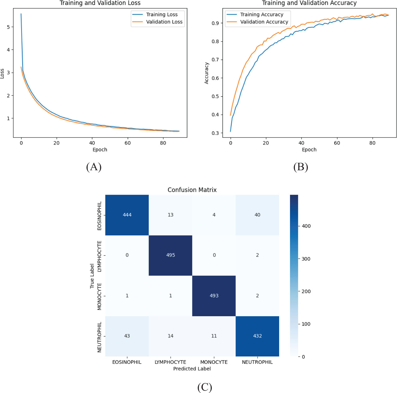
Figure 17:
(A) presents the accuracy of training and validation for each epoch, (B) illustrates the loss during training and validation for each epoch, and (C) shows the confusion matrix for each class from the VGG16 Model.
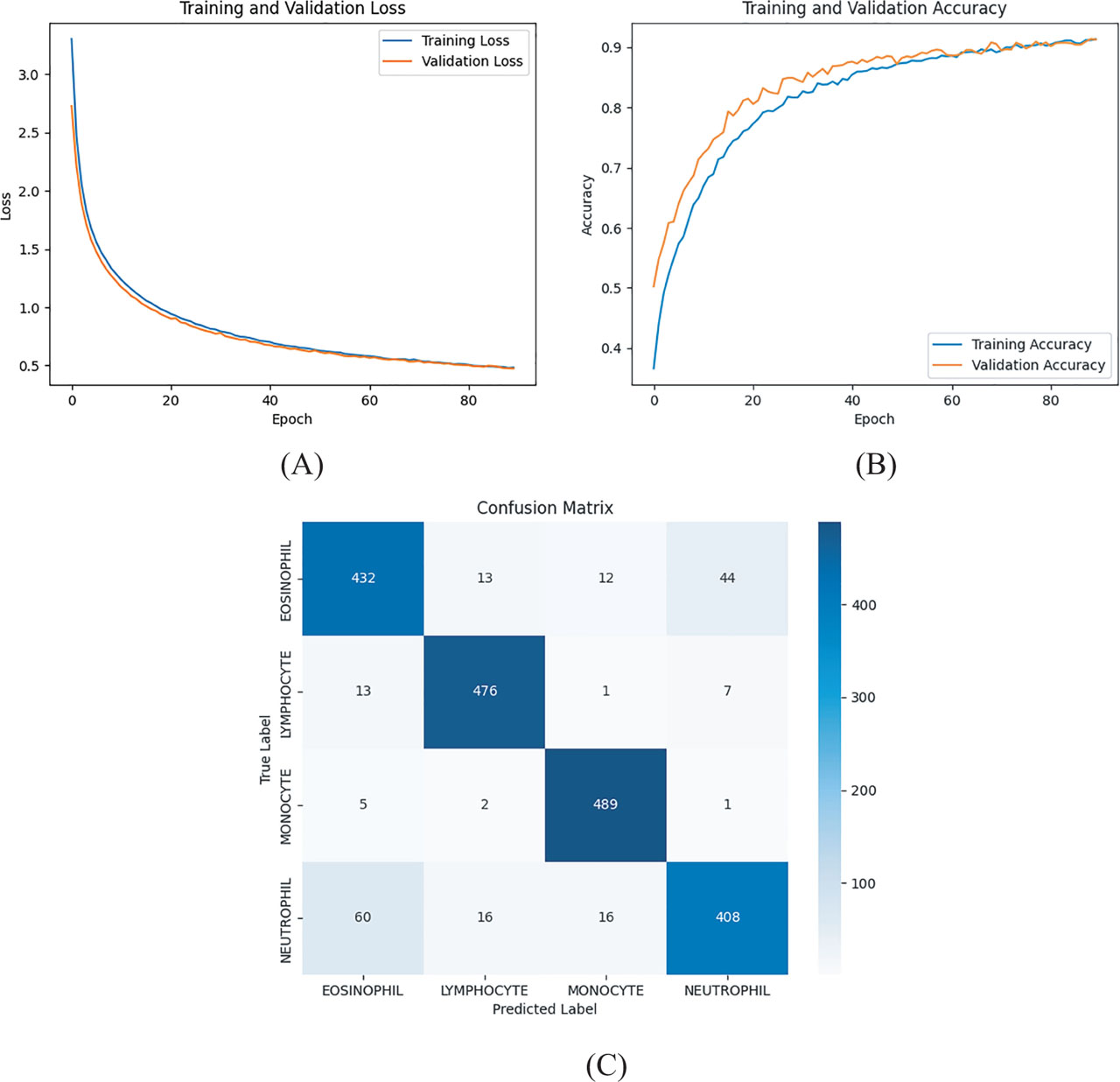
Figure 18:
(A) presents the training and validation accuracy per epoch, (B) shows the training and validation loss for each epoch, and (C) provides the confusion matrix for each class from the DenseNET121 model.