
Table 1.
Mathematical models for PQDs and relevant parameters.
| PQ disturbance | Class | Equations | Parameters |
|---|---|---|---|
| Normal voltage | C0 | α < 0.1 | |
| Sag | C1 | 0.16 ≤ α ≤ 0.23 | |
| Swell | C2 | 0.2 ≤ α ≤ 0.28 | |
| Interruption | C3 | 0.075 < α ≤ 0.2 | |
| Harmonics | C4 | 0 ″ hi ″ 0.15 | |
| Flicker | C5 | αf = 0.1 − 0.15, βf = 5 − 7.5 | |
| Sag with harm | C6 | 0.05 ≤ α ≤ 0.15 | |
| Swell with harm | C7 | 01. ≤ α ≤ 0.18 | |
| Oscillatory transient | C8 | 0.1 < β < 0.8,0.066 < τ 0.008 ωn = 2π fn, 500 ≤ fn ≤ 1500 |
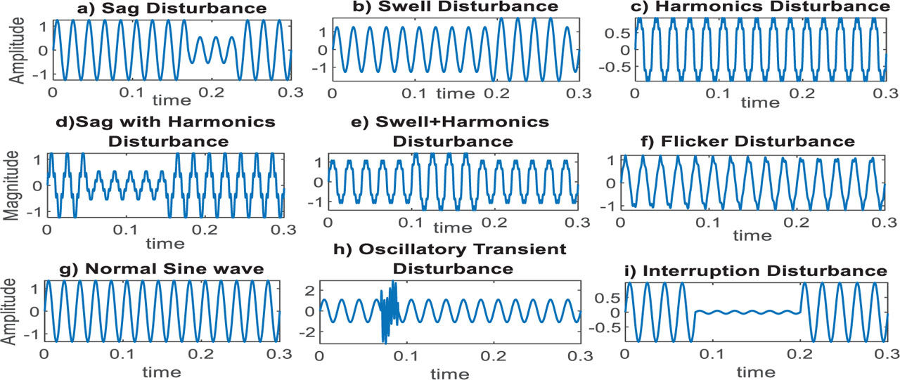
Figure 1:
PQD signal models covering all types of disturbance signals (stationary and nonstationary) included normal sine waves.
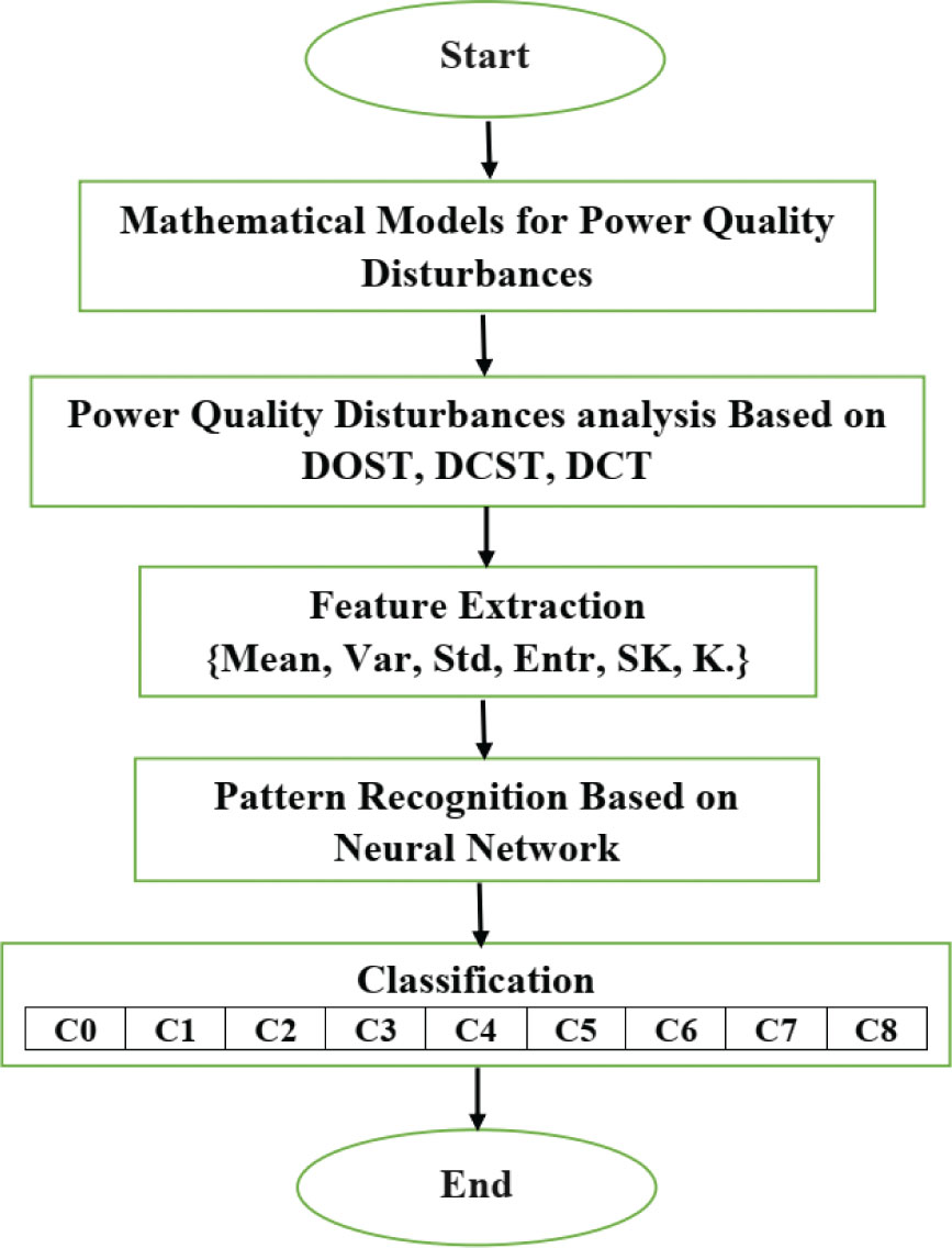
Figure 2:
Flowchart of the PQD analysis and classification system.
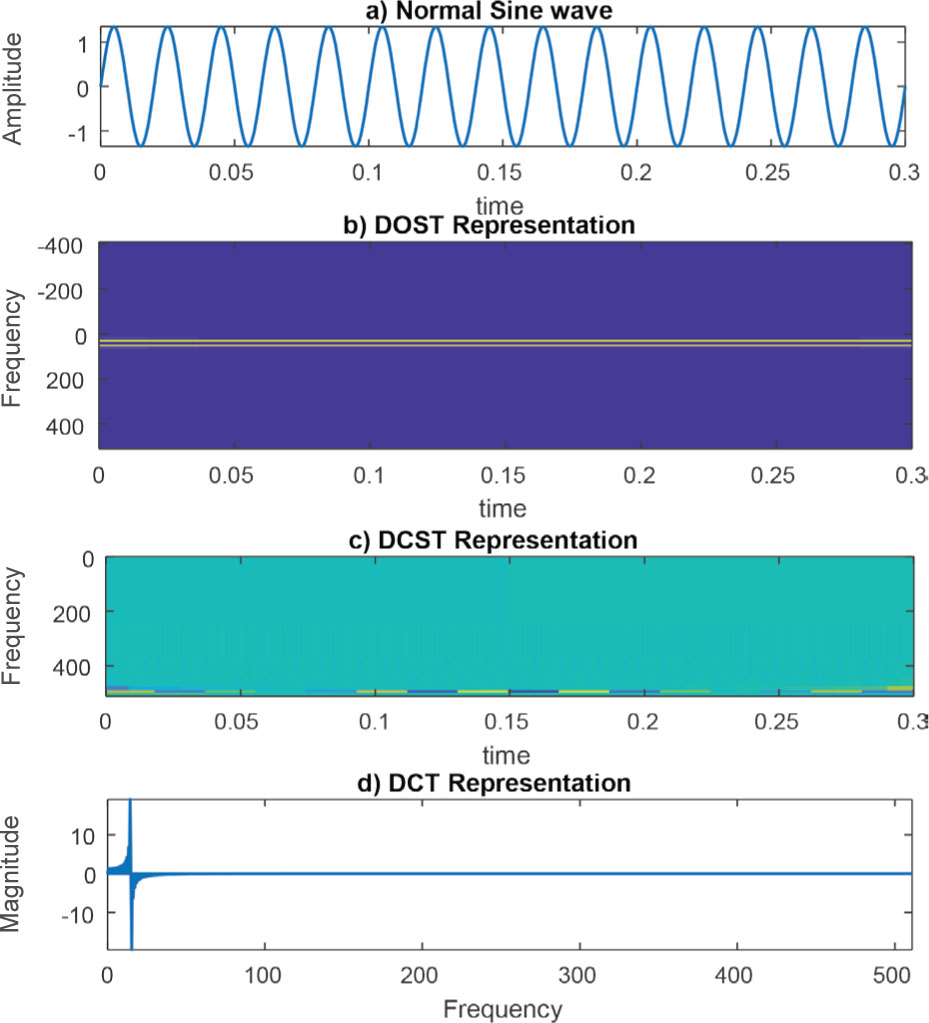
Figure 3:
Normal sine wave: (a) target disturbance – nonstationary signal (clean and stable sine wave without any disturbance) for all methods, (b) DOST, (c) DCST, and (d) DCT.
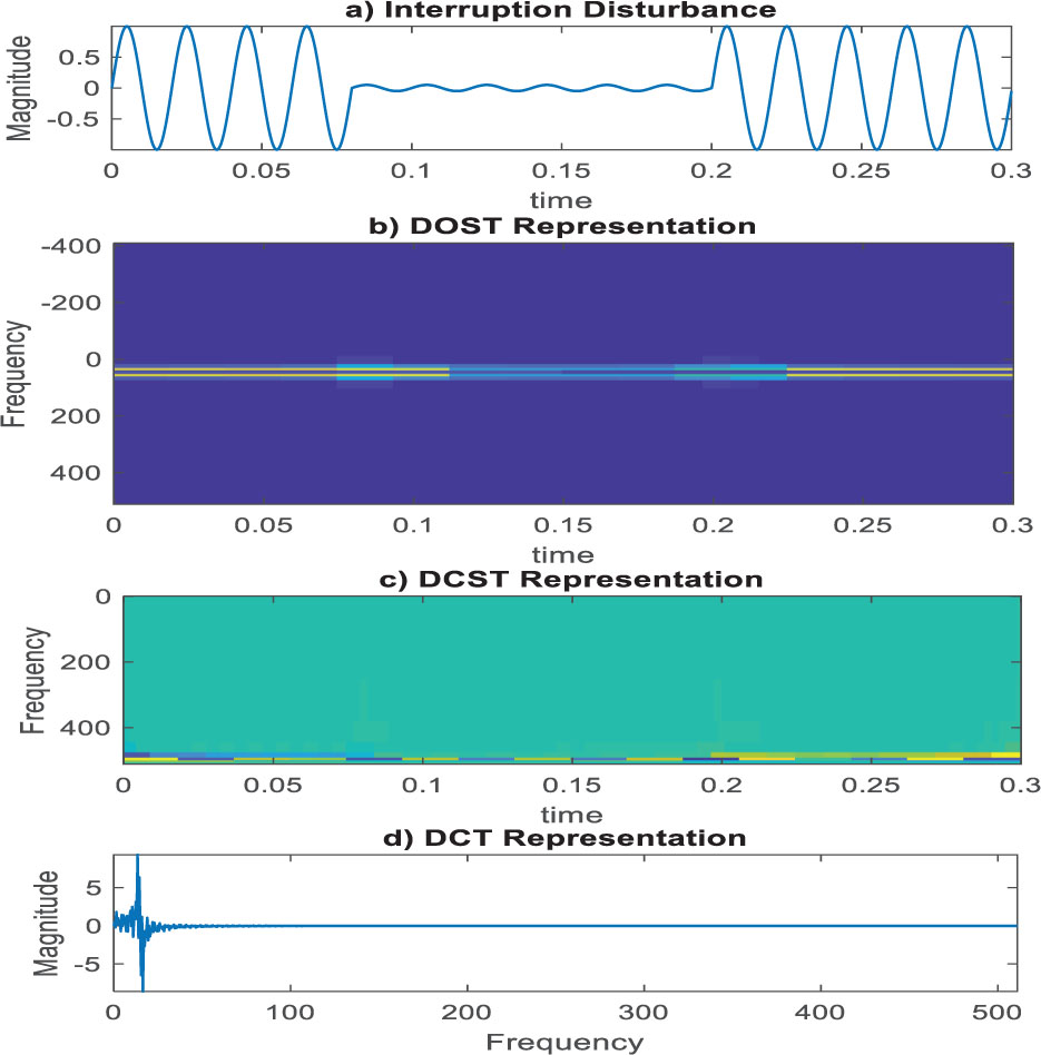
Figure 4:
Interruption disturbance signal: (a) target disturbance – nonstationary signal (from 0.075 s to 0.2 s) for all methods. Intended coefficients of the time and frequency fluctuations, including amplitude and angle, for all methods; (b) DOST – the signal time interval corresponds to the target signal and works to accurately capture localized changes in signal characteristics; (c) DCST – some effects on the windows; and (d) DCT – much more limited frequency resolution compared with other time–frequency analytic methods but may capture a few fine-frequency details in the PQDs.
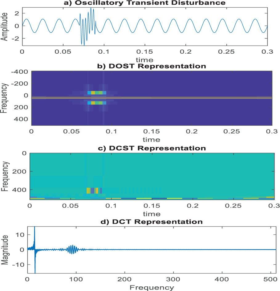
Figure 5:
Oscillatory transient disturbance signal: (a) target disturbance – nonstationary signal and its corresponding Stockwell transform-based methods, in which disturbance in all plots occurs at 0.066–0.08 s; (b) DOST – may exhibit better noise robustness than other time–frequency analytic techniques, resulting in cleaner and clearer plotting of PQDs even in the presence of noise or interference; (c) DCST – frequency magnitude increased to 400 Hz corresponding to the time disturbance interval in (b); and (d) DCT – rising multiples in these disturbances, from 0 Hz to 105 Hz, with inter-harmonic and harmonic features.
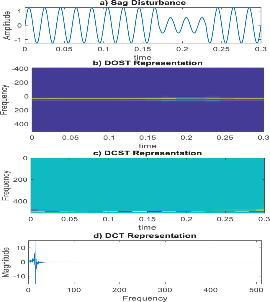
Figure 6:
Sag disturbance signal: (a) target disturbance – stationary signal and its corresponding plots allow each method to perform excellently, with the disturbance occurring from 0.16 s to 0.23 s; the intended coefficients of both time and frequency fluctuations, including amplitude and angle, for all methods. (b) DOST – sag effects with a corresponding rate of 100%. (c) DCST – moderate resolution may not capture all of the fine details for certain PQDs with rapidly changing characteristics, leading to less clear plots. (d) DCT – operates on discrete data points and assumes the signal to be periodic; this discrete nature may lead to artifacts in the time–frequency representation, affecting the clarity of the plots.
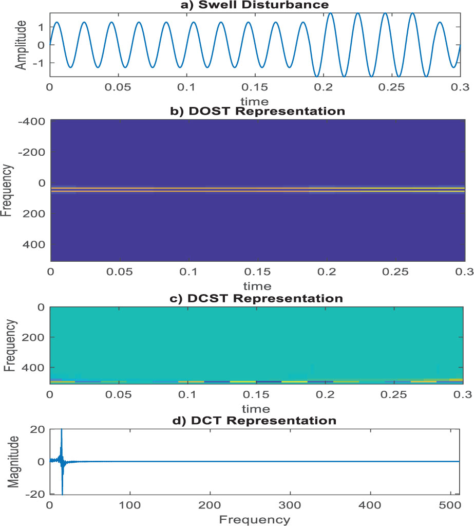
Figure 7:
Swell disturbance signal: (a) target disturbance – a stationary signal and represented by all methods, with disturbance occurring from 0.2 s to 0.28 s; the intended coefficients of both time and frequency fluctuations, including amplitude and angle, for all methods. (b) DOST, (c) DCST, and (d) DCT – depend on the specific characteristics of the simulated PQDs. For disturbances with complex or rapidly changing time–frequency components, the DCT may not be the most suitable method, despite its simple but precise plots.
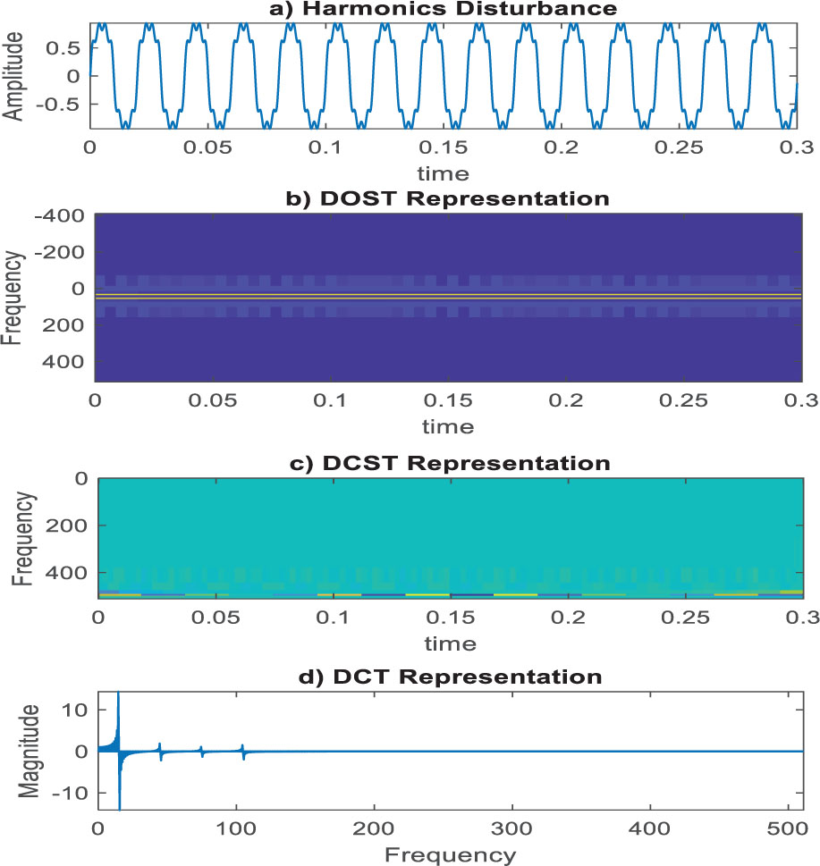
Figure 8:
Harmonic disturbance signal: (a) target signal – a stationary signal; the intended coefficients of both time and frequency fluctuations, including amplitude and angle, for all methods. (b) DOST time–frequency representation – ability to represent stationary and nonstationary signals, contributing to the clear plotting of disturbances. (c) DCST time–frequency representation. (d) DCT – known for its energy compaction properties, in which a large portion of the signal energy is concentrated in a few DCT coefficients; this method can result in some aspects of the disturbances being well represented, while others are not.
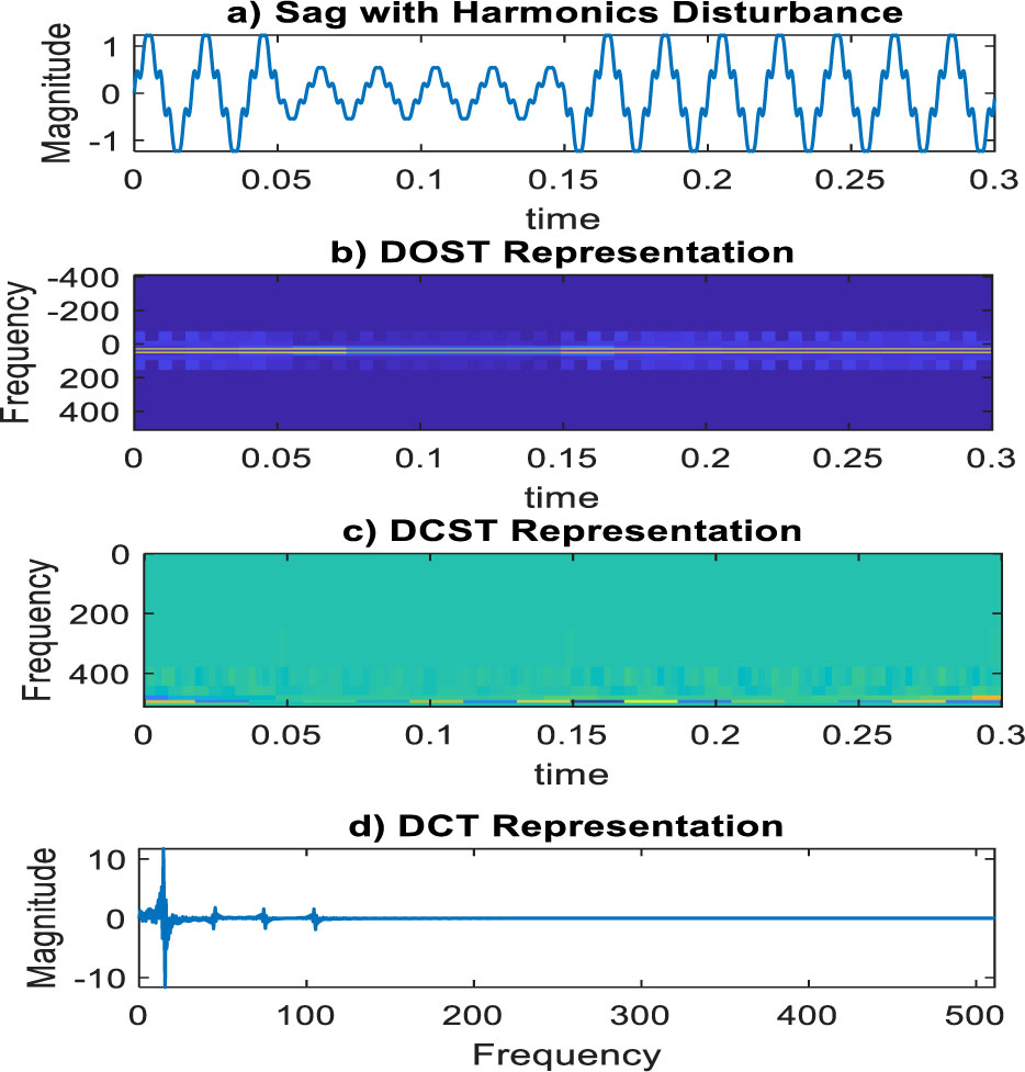
Figure 9:
Sag with harmonics disturbance signal: (a) target signal – a stationary signal (from 0.05 s to 0.15 s); the intended coefficients of both time and frequency fluctuation, including amplitude and angle, for all methods. (b) DOST representation – uses different windowing functions in which a selected appropriate window can enhance the clarity of the plot by minimizing spectral leakage and side lobe effects. (c) DCST representation. (d) DCT representation – the rising multiple effective in this type of disturbance (inter-harmonics and harmonics: 25, 50, 75, and 104 Hz).
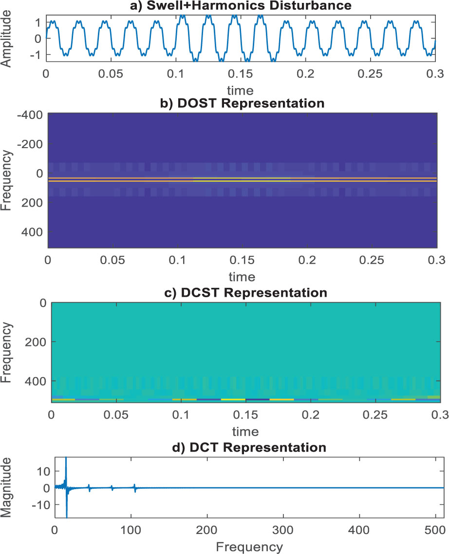
Figure 10:
Swell with a harmonic disturbance signal: (a) target signal – a stationary signal from 0.1 s to 0.18 s; the intended coefficients of both time and frequency fluctuation, including amplitude and angle, for all methods. (b) DOST time–frequency representation. (c) DCST representation. (d) DCT representation.
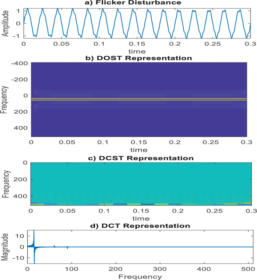
Figure 11:
Flicker disturbance signal: (a) original signal – a stationary signal; the intended coefficients of both time and frequency fluctuation, including amplitude and angle, for all methods. (b) DOST, (c) DCST, and (d) DCT – the rising multiple effectiveness in these types of disturbances (25, 75, and 99 Hz for inter-harmonics and harmonics).
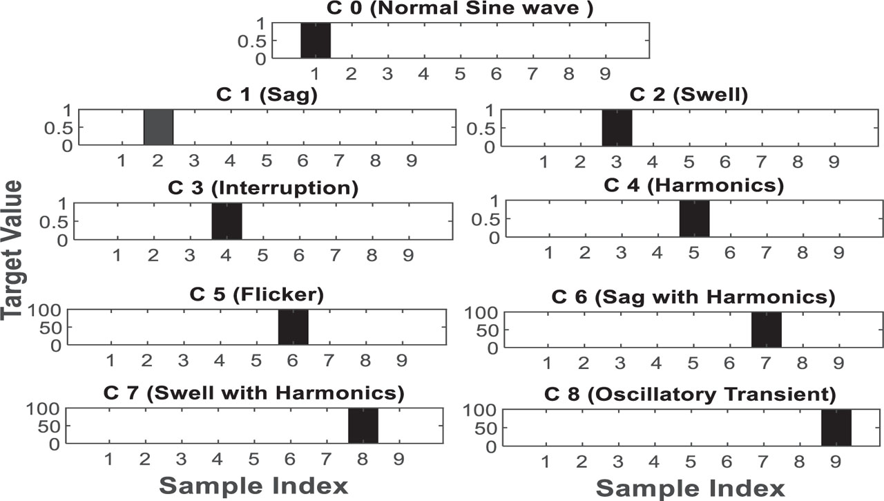
Figure 12:
Disturbance classification-based statistical analysis (mean, variation, standard deviation, entropy, skewness, and kurtosis) of the DOST, DCST, and DCT coefficients.
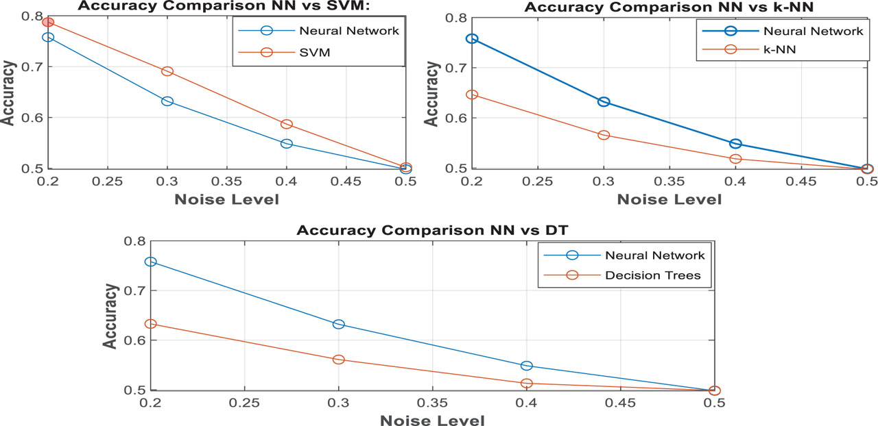
Figure 13:
Accuracy comparison between the neural network method and SVM, KNN, and DT.
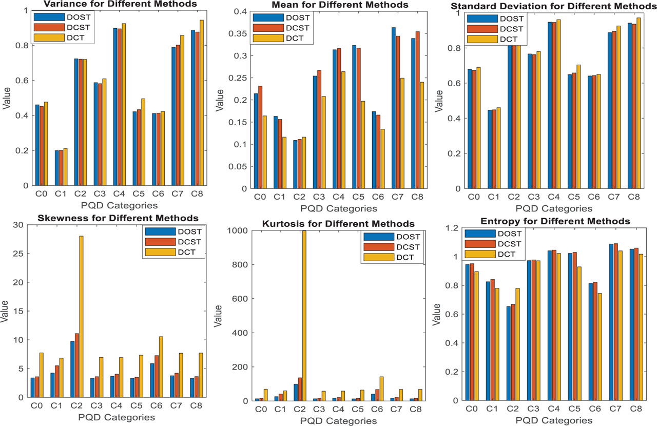
Figure 14:
Statistical analysis features properties’ comparison (mean, variation, standard deviation, entropy, skewness, and kurtosis) of DOST, DCST, and DCT coefficients.