
Table 1
Quantitative assessment of solution accuracy: Comparison of analytical solutions obtained via the 𝕀𝕂ud method including tabulated values of analytical solutions, numerical solutions, and absolute errors at specified intervals.
| Value of (x) | Ex. Sol. | Com. Sol. | |Error| |
|---|---|---|---|
| 0.03125 | 1.20763958026872 | 1.20763958031072 | 4.20047074605165E-11 |
| 0.046875 | 1.21674003497737 | 1.21674003502882 | 5.14567661613503E-11 |
| 0.0625 | 1.22575976468092 | 1.22575976474224 | 6.13197720729986E-11 |
| 0.078125 | 1.23469622228169 | 1.23469622235328 | 7.15925370223830E-11 |
| 0.09375 | 1.24354695100228 | 1.24354695108456 | 8.22729750443174E-11 |
| 0.109375 | 1.25230958756389 | 1.25230958765725 | 9.33581005884076E-11 |
| 0.125 | 1.26098186511128 | 1.26098186521613 | 1.04844030930955E-10 |
| 0.140625 | 1.26956161587652 | 1.26956161599325 | 1.16725992784197E-10 |
| 0.15625 | 1.27804677357473 | 1.27804677370373 | 1.28998333062043E-10 |
| 0.171875 | 1.28643537552652 | 1.28643537566817 | 1.41654533728808E-10 |
| 0.1875 | 1.29472556450305 | 1.29472556465774 | 1.54687230625832E-10 |
| 0.203125 | 1.30291559029133 | 1.30291559045942 | 1.68088236140455E-10 |
| 0.21875 | 1.31100381097824 | 1.31100381116009 | 1.81848565553179E-10 |
| 0.234375 | 1.31898869395364 | 1.31898869414960 | 1.95958466872067E-10 |
| 0.25 | 1.32686881663397 | 1.32686881684438 | 2.10407453938981E-10 |
| 0.265625 | 1.33464286690894 | 1.33464286713413 | 2.25184342570225E-10 |
| 0.28125 | 1.34230964331548 | 1.34230964355576 | 2.40277289474885E-10 |
| 0.296875 | 1.34986805494397 | 1.34986805519964 | 2.55673833677647E-10 |
| 0.3125 | 1.35731712108310 | 1.35731712135446 | 2.71360940159403E-10 |
| 0.328125 | 1.36465597061072 | 1.36465597089804 | 2.87325045418458E-10 |
| 0.34375 | 1.37188384113887 | 1.37188384144243 | 3.03552104647745E-10 |
| 0.359375 | 1.37900007792241 | 1.37900007824244 | 3.20027640219087E-10 |
| 0.375 | 1.38600413254102 | 1.38600413287775 | 3.36736791164162E-10 |
| 0.390625 | 1.39289556136557 | 1.39289556171923 | 3.53664363343354E-10 |
| 0.40625 | 1.39967402382009 | 1.39967402419088 | 3.70794879997960E-10 |
| 0.421875 | 1.40633928045129 | 1.40633928083940 | 3.88112632388131E-10 |
| 0.4375 | 1.41289119081811 | 1.41289119122371 | 4.05601730228252E-10 |
| 0.453125 | 1.41932971121393 | 1.41932971163717 | 4.23246151643027E-10 |
| 0.46875 | 1.42565489223455 | 1.42565489267558 | 4.41029792381063E-10 |
| 0.484375 | 1.43186687620519 | 1.43186687666413 | 4.58936514038058E-10 |
Table 2
Quantitative assessment of solution accuracy: Comparison of analytical solutions obtained with numerical solutions computed using the ℍ𝕍𝕀 technique, including tabulated values of analytical solutions, numerical solutions, and absolute errors at specified intervals.
| Value of (x) | Ex. Sol. | Com. Sol. | |Error| |
|---|---|---|---|
| 0.546875 | 1.45558874428203 | 1.45558874481351 | 5.31472836811428E-10 |
| 0.5625 | 1.46123989332295 | 1.46123989387271 | 5.49754896154283E-10 |
| 0.578125 | 1.46678046707451 | 1.46678046764258 | 5.68065010144654E-10 |
| 0.59375 | 1.47221116886342 | 1.47221116944981 | 5.86388024555344E-10 |
| 0.609375 | 1.47753276966930 | 1.47753277027401 | 6.04709077390241E-10 |
| 0.625 | 1.48274610486957 | 1.48274610549258 | 6.23013630104608E-10 |
| 0.640625 | 1.48785207096936 | 1.48785207161065 | 6.41287496403386E-10 |
| 0.65625 | 1.49285162232708 | 1.49285162298659 | 6.59516868582952E-10 |
| 0.671875 | 1.49774576788572 | 1.49774576856341 | 6.77688341399560E-10 |
| 0.6875 | 1.50253556791965 | 1.50253556861544 | 6.95788933464592E-10 |
| 0.703125 | 1.50722213080576 | 1.50722213151957 | 7.13806106182524E-10 |
| 0.71875 | 1.51180660982761 | 1.51180661055933 | 7.31727780262184E-10 |
| 0.734375 | 1.51629020002027 | 1.51629020076982 | 7.49542349845331E-10 |
| 0.75 | 1.52067413506334 | 1.52067413583058 | 7.67238694308809E-10 |
| 0.765625 | 1.52495968422856 | 1.52495968501337 | 7.84806187807455E-10 |
| 0.78125 | 1.52914814938845 | 1.52914815019068 | 8.02234706634669E-10 |
| 0.796875 | 1.53324086209117 | 1.53324086291068 | 8.19514634485941E-10 |
| 0.8125 | 1.53723918070676 | 1.53723918154340 | 8.36636865717824E-10 |
| 0.828125 | 1.54114448764904 | 1.54114448850264 | 8.53592806700824E-10 |
| 0.84375 | 1.54495818667699 | 1.54495818754737 | 8.70374375369481E-10 |
| 0.859375 | 1.54868170027898 | 1.54868170116595 | 8.86973999076636E-10 |
| 0.875 | 1.55231646714259 | 1.55231646804597 | 9.03384610861484E-10 |
| 0.890625 | 1.55586393971231 | 1.55586394063191 | 9.19599644242735E-10 |
| 0.90625 | 1.55932558183708 | 1.55932558277269 | 9.35613026648884E-10 |
| 0.921875 | 1.56270286650881 | 1.56270286746023 | 9.51419171597521E-10 |
| 0.9375 | 1.56599727369322 | 1.56599727466023 | 9.67012969734731E-10 |
| 0.953125 | 1.56921028825326 | 1.56921028923565 | 9.82389778844027E-10 |
| 0.96875 | 1.57234339796551 | 1.57234339896306 | 9.97545412932099E-10 |
| 0.984375 | 1.57539809162942 | 1.57539809264189 | 1.01247613049587E-09 |
| 1 | 1.57837585726886 | 1.57837585829604 | 1.02717862207213E-09 |
Table 3
Quantitative evaluation of solution accuracy entails comparing analytical solutions obtained from the 𝕄ℝat. This comparison involves tabulating values of analytical solutions, numerical solutions, and absolute errors at specified intervals.
| Value of (x) | Ex. Sol. | Com. Sol. | |Error| |
|---|---|---|---|
| 0 | 0.99999999990000 | 0.99999999990000 | 4.99999999916667E-21 |
| 0.015625 | 1.02315233356186 | 1.02315233360905 | 4.71888812971725E-11 |
| 0.03125 | 1.04569417315531 | 1.04569417325986 | 1.04543443435149E-10 |
| 0.046875 | 1.06756981159651 | 1.06756981176867 | 1.72151359548055E-10 |
| 0.0625 | 1.08873008579492 | 1.08873008604480 | 2.49886490304410E-10 |
| 0.078125 | 1.10913286437772 | 1.10913286471513 | 3.37410497362432E-10 |
| 0.09375 | 1.12874336710157 | 1.12874336753575 | 4.34183467238255E-10 |
| 0.109375 | 1.14753431362354 | 1.14753431416302 | 5.39482727708055E-10 |
| 0.125 | 1.16548590646840 | 1.16548590712083 | 6.52428510356929E-10 |
| 0.140625 | 1.18258565945528 | 1.18258566022729 | 7.72014729099501E-10 |
| 0.15625 | 1.19882808816775 | 1.19882808906489 | 8.97142932229239E-10 |
| 0.171875 | 1.21421428302518 | 1.21421428405184 | 1.02665744908632E-09 |
| 0.1875 | 1.22875138803065 | 1.22875138919003 | 1.15937987555944E-09 |
| 0.203125 | 1.24245200934976 | 1.24245201064391 | 1.29414129352527E-09 |
| 0.21875 | 1.25533357764067 | 1.25533357907048 | 1.42981095696222E-09 |
| 0.234375 | 1.26741768671079 | 1.26741768827611 | 1.56532055830938E-09 |
| 0.25 | 1.27872942887382 | 1.27872943057351 | 1.69968357236353E-09 |
| 0.265625 | 1.28929674458767 | 1.28929674641968 | 1.83200952868107E-09 |
| 0.28125 | 1.29914980083272 | 1.29914980279423 | 1.96151336375456E-09 |
| 0.296875 | 1.30832040947003 | 1.30832041155755 | 2.08752023792844E-09 |
| 0.3125 | 1.31684149369319 | 1.31684149590266 | 2.20946636502446E-09 |
| 0.328125 | 1.32474660780002 | 1.32474661012692 | 2.32689649821843E-09 |
| 0.34375 | 1.33206951295875 | 1.33206951539821 | 2.43945875222451E-09 |
| 0.359375 | 1.33884380948371 | 1.33884381203061 | 2.54689743060630E-09 |
| 0.375 | 1.34510262438699 | 1.34510262703604 | 2.64904448037841E-09 |
| 0.390625 | 1.35087835162533 | 1.35087835437114 | 2.74581012589749E-09 |
| 0.40625 | 1.35620244148743 | 1.35620244432460 | 2.83717315088190E-09 |
| 0.421875 | 1.36110523492245 | 1.36110523784562 | 2.92317120983896E-09 |
| 0.4375 | 1.36561583824674 | 1.36561584125063 | 3.00389146472270E-09 |
| 0.453125 | 1.36976203353220 | 1.36976203661166 | 3.07946176379683E-09 |
| 0.46875 | 1.37357022002564 | 1.37357022317569 | 3.15004251018863E-09 |
| 0.484375 | 1.37706538213010 | 1.37706538534592 | 3.21581930881469E-09 |
Table 4
Quantitative evaluation of solution accuracy entails comparing analytical solutions obtained with numerical solutions computed using the ℍ𝕍𝕀 technique. This comparison involves tabulating values of analytical solutions, numerical solutions, and absolute errors at specified intervals.
| Value of (x) | Ex. Sol. | Com. Sol. | |Error| |
|---|---|---|---|
| 0.515625 | 1.38320945718246 | 1.38320946051625 | 3.33379111053848E-09 |
| 0.53125 | 1.38590126696226 | 1.38590127034869 | 3.38642861532610E-09 |
| 0.546875 | 1.38836590574752 | 1.38836590918266 | 3.43513810202309E-09 |
| 0.5625 | 1.39062145934722 | 1.39062146282737 | 3.48014914421751E-09 |
| 0 0.578125 | 1.39268475465260 | 1.39268475817429 | 3.52168890024829E-09 |
| 0.59375 | 1.39457141643050 | 1.39457141999048 | 3.55997984207624E-09 |
| 0.609375 | 1.39629592729448 | 1.39629593088972 | 3.59523797853094E-09 |
| 0.625 | 1.39787168944864 | 1.39787169307631 | 3.62767150716086E-09 |
| 0.640625 | 1.39931108705224 | 1.39931109070972 | 3.65747983287765E-09 |
| 0.65625 | 1.40062554827592 | 1.40062555196077 | 3.68485289652858E-09 |
| 0.671875 | 1.40182560631267 | 1.40182561002264 | 3.70997076199180E-09 |
| 0.6875 | 1.40292095877275 | 1.40292096250575 | 3.73300341601893E-09 |
| 0.703125 | 1.40392052503188 | 1.40392052878600 | 3.75411074059905E-09 |
| 0.71875 | 1.40483250122032 | 1.40483250499377 | 3.77344262291369E-09 |
| 0.734375 | 1.40566441263838 | 1.40566441642952 | 3.79113917288493E-09 |
| 0.75 | 1.40642316346472 | 1.40642316727205 | 380733102282274E-09 |
| 0.765625 | 1.40711508368922 | 1.40711508751136 | 3.82213968772653E-09 |
| 0.78125 | 1.40774597325455 | 1.40774597709023 | 3.83567796838594E-09 |
| 0.796875 | 1.40832114343230 | 1.40832114728035 | 3.84805038257160E-09 |
| 0.8125 | 1.40884545549122 | 1.40884545935057 | 3.85935361233518E-09 |
| 0.828125 | 1.40932335673971 | 1.40932336060938 | 3.86967695778105E-09 |
| 0.84375 | 1.40975891404212 | 1.40975891792122 | 3.87910278966745E-09 |
| 0.859375 | 1.41015584492121 | 1.41015584880892 | 3.88770699487884E-09 |
| 0.875 | 1.41051754636684 | 1.41051755026240 | 3.89555941022204E-09 |
| 0.890625 | 1.41084712147580 | 1.41084712537852 | 3.90272424116893E-09 |
| 0.90625 | 1.41114740404942 | 1.41114740795868 | 3.90926046313347E-09 |
| 0.921875 | 1.41142098127513 | 1.41142098519035 | 3.91522220365665E-09 |
| 0.9375 | 1.41167021461611 | 1.41167021853677 | 3.92065910450927E-09 |
| 0.953125 | 1.41189725902987 | 1.41189726295548 | 3.92561666322989E-09 |
| 00.96875 | 1.41210408063213 | 1.41210408456227 | 3.93013655401647E-09 |
| 0.984375 | 1.41229247291764 | 1.41229247685190 | 3.93425692820126E-09 |
| 1 | 1.41246407164386 | 1.41246407558187 | 3.93801269477613E-09 |
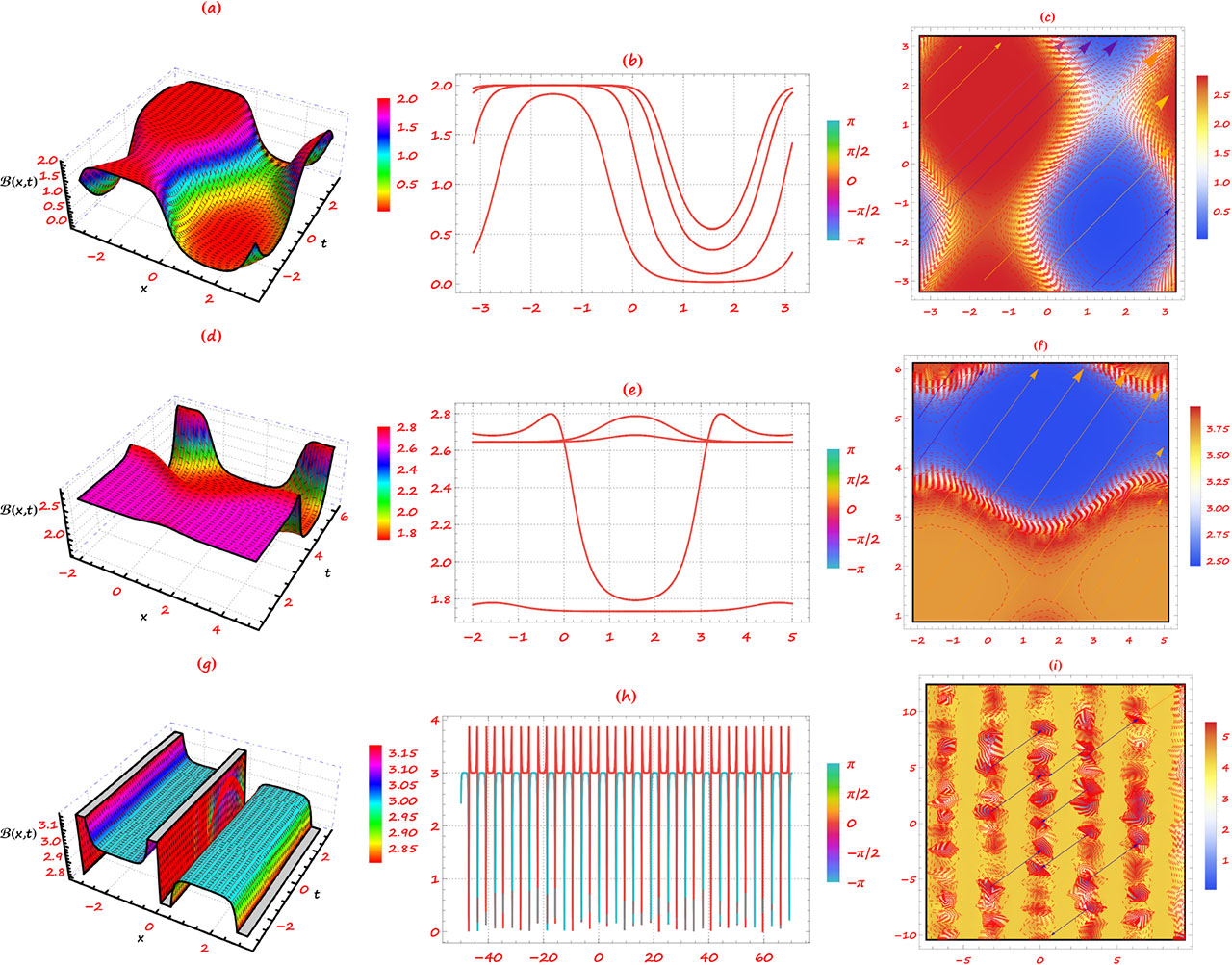
Fig. 1
Graphical representations of analytical solitary wave solutions to the nonlinear 𝕂𝔾 equation, obtained via the 𝕀𝕂ud method.
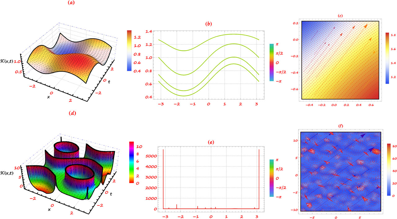
Fig. 2
Graphical illustrations of analytical solitary wave solutions to the nonlinear 𝕂𝔾 equation, obtained through the 𝕄ℝat method.
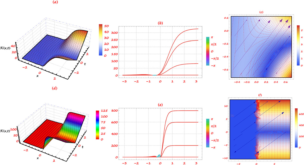
Fig. 3
Graphical representations of numerical solutions to the nonlinear Klein-Gordon equation, obtained via the ℍ𝕍𝕀 method.
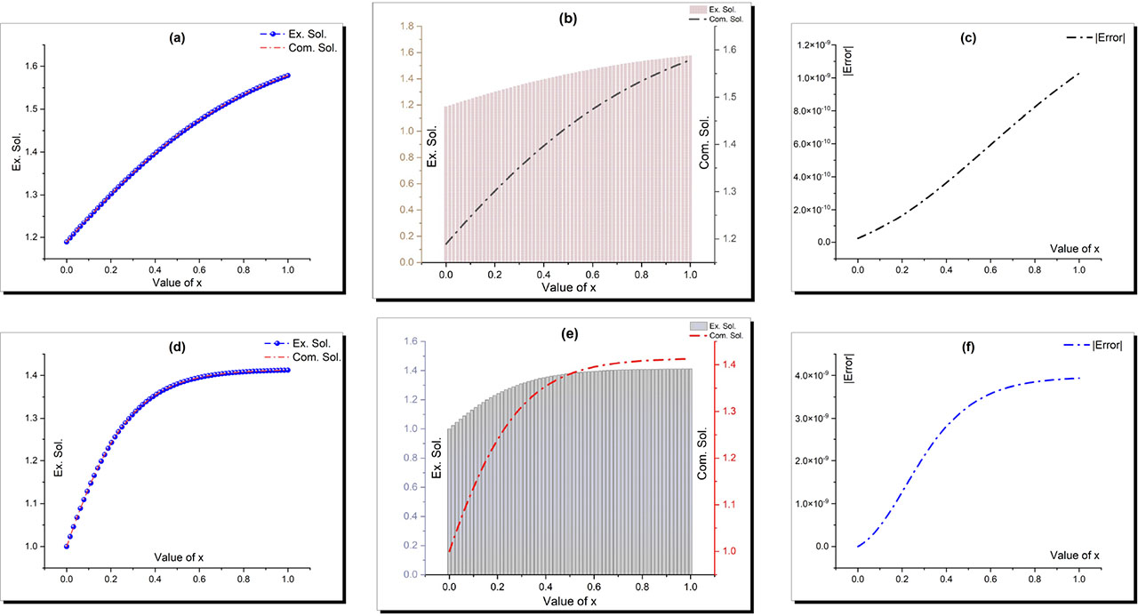
Fig. 4
Quantitative validation of analytical solutions against numerical solutions through absolute error analysis.
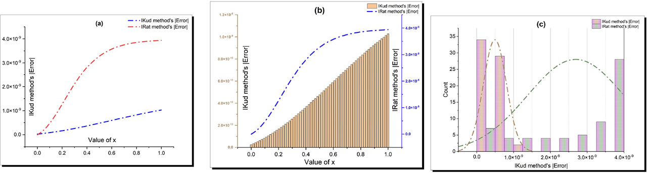
Fig. 5
Comparative assessment of solution accuracy for the 𝕀𝕂ud and 𝕄ℝat analytical techniques, bench-marked against ℍ𝕍𝕀 numerical solutions.
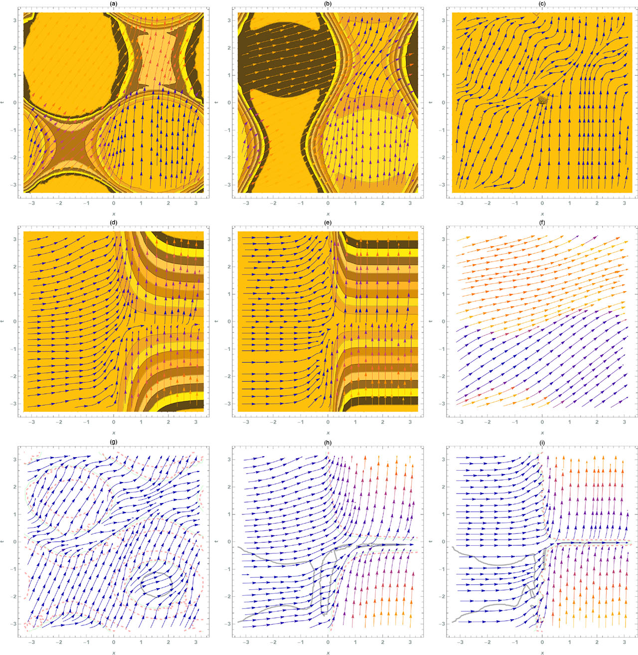
Fig. 6
Stream plot depicting the interaction of multiple solitary waves within the nonlinear 𝕂𝔾 model.
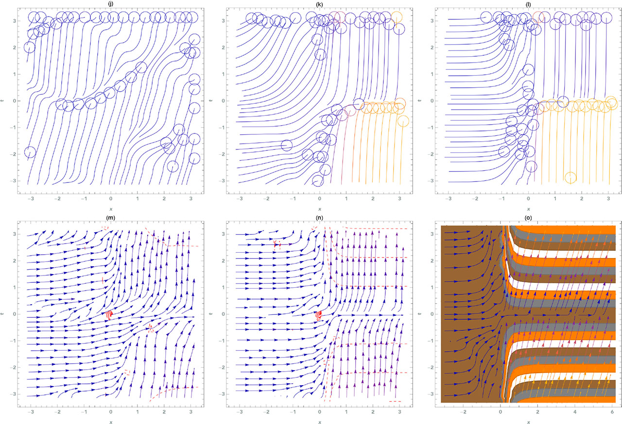
Fig. 7
Stream plot illustrating the propagation of solitary waves generated by the nonlinear 𝕂𝔾 model.