
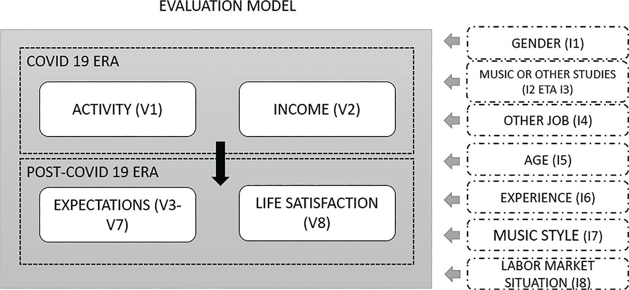
Figure 1.
Evaluation model.
Table 1.
Independent variables (general characteristics).
| I1 | Gender |
| I2 | Music studies |
| I3 | Other studies |
| I4 | Age |
| I5 | Experience |
| I6 | Other job |
| I7 | Music style |
| I8 | Labour market situation |
Table 2.
Dependent variables.
| V1 | Impact of COVID-19 on own musical activity |
| V2 | Impact of COVID-19 on income |
| V3 | Expectations regarding income recovery in 2021 and beyond |
| V4 | Expectations regarding carrying on with same type of musical employment in 2021 and beyond |
| V5 | Expectations regarding carrying on with any type of musical employment in 2021 and beyond |
| V6 | Expectations regarding a recovery of the demand of own musical activity in 2021 and beyond |
| V7 | Expectations regarding a recovery of the demand of live concerts in 2021 and beyond |
| V8 | General life satisfaction |
[i] All these variables are ordinal variables. Variables 1 and 2 offered five possible answers. While the answers for Variable 1 (effect of COVID-19 on music activity) ranged from “very positive” (1), to “very negative” (5), answers to Variable 2 (impact of COVID-19 on income) ranged from an income loss between 0% and 20% (1) to an income loss between 81% and 100% (5). V3–V8 offered ten possible answers (being 1 = very low, and 10 = very high).
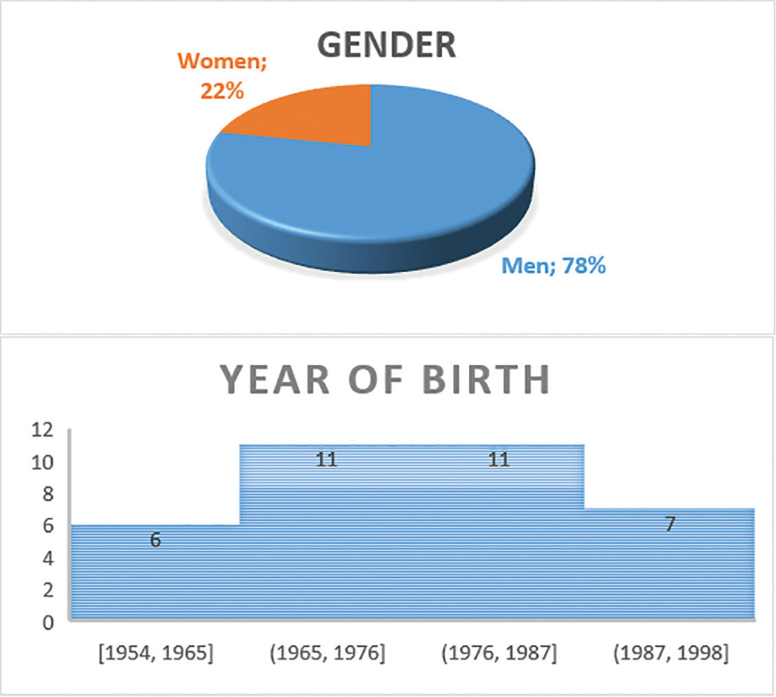
Figure 2.
Gender and year of birth.
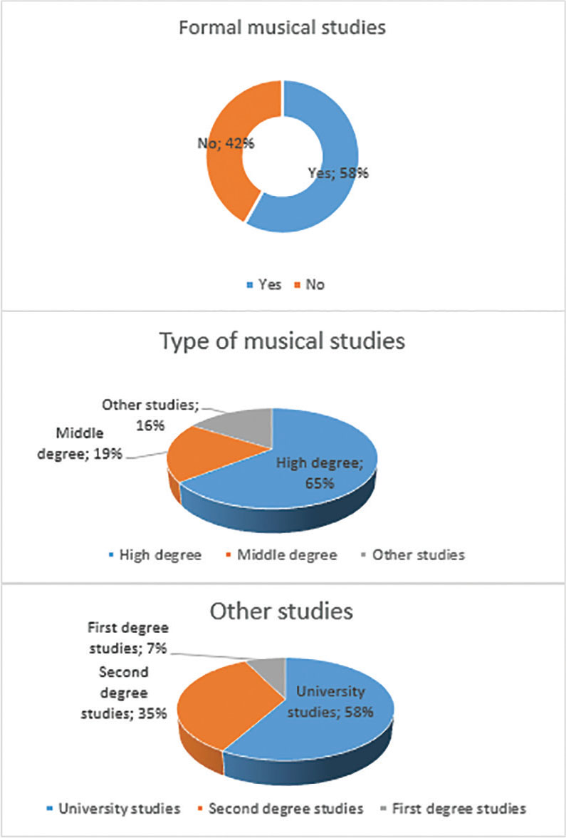
Figure 3.
Musical and other studies.
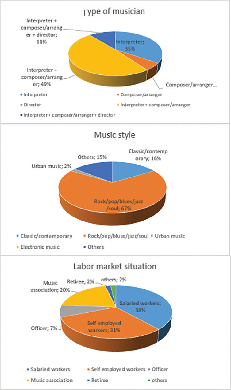
Figure 4.
Type of musician, music style and labour market situation.
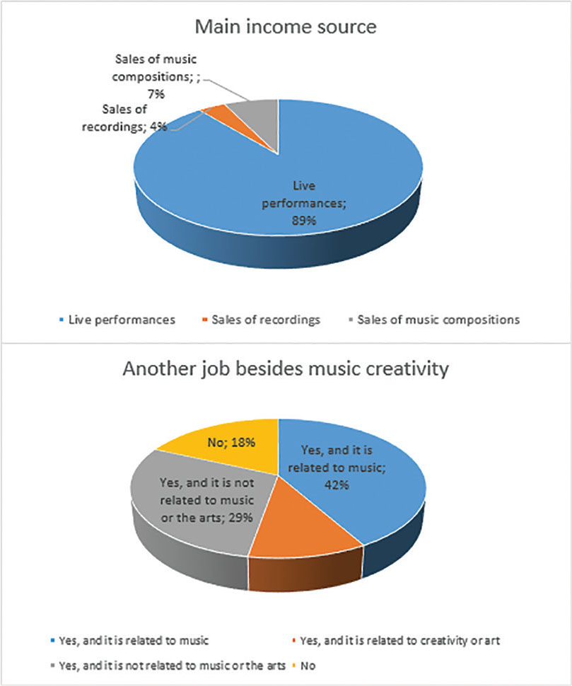
Figure 5.
Main income source and other job.
Table 3.
Correlation rates (independent variables – V1, V2).
| I1 | I2 | I3 | I4 | I5 | I6 | I7 | I8 | |
|---|---|---|---|---|---|---|---|---|
| V1 | −0.096 | 0.145 | −0.159 | −0.042 | −0.168 | 0.026 | −0.101 | 0.116 |
| V2 | −0.113 | 0.044 | 0.028 | 0.007 | −0.035 | 0.168 | 0.100 | −0.035 |

Figure 6.
Impact of COVID-19 on music activity and income.
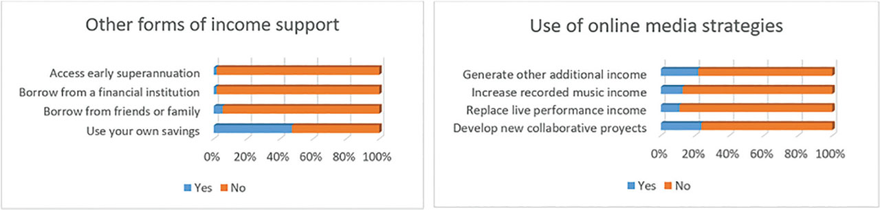
Figure 7.
Form of income support and new online media strategies..
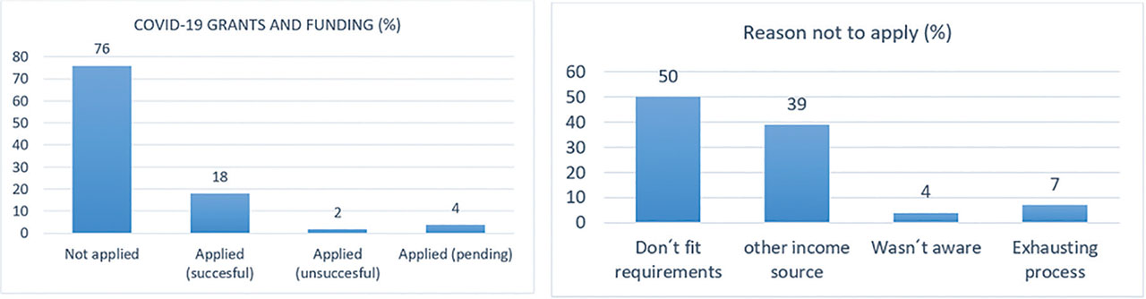
Figure 8.
COVID-19 grants and funding.
Table 4.
Correlation rates (independent variables – V3–V8).
| I1 | I2 | I3 | I4 | I5 | I6 | I7 | I8 | |
|---|---|---|---|---|---|---|---|---|
| V3 | −0.212 | −0.288* | −0.013 | 0.145 | 0.102 | −0.095 | −0.130 | −0.034 |
| V4 | −0.136 | −0.202 | −0.29 | 0.296* | 0.269* | −0.093 | −0.241 | 0.109 |
| V5 | −0.299* | 0.084 | −0.012 | 0.145 | 0.202 | −0.049 | −0.074 | 0.114 |
| V6 | −0.229 | −0.394** | −0.158 | 0.084 | 0.155 | −0.219 | −0.123 | −0.152 |
| V7 | −0.203 | −0.350** | −0.172 | −0.019 | 0.125 | −0.332* | −0.055 | −0.106 |
| V8 | −0.306* | −0.039 | −0.034 | −0.077 | −0.083 | −0.122 | −0.135 | −0.045 |
Table 5.
Inference main results.
| Independent variable | Hypothesis | Affected variable | Sig. level | |
|---|---|---|---|---|
| I1 | Gender | H1 | V5 | 0.028 |
| H2 | V8 | 0.025 | ||
| I2 | Music studies | H3 | V3 | 0.035 |
| H4 | V6 | 0.04 | ||
| H5 | V7 | 0.01 | ||
| I4 | Other job | H6 | V7 | 0.013 |
| I5 | Age | H7 | V4 | 0.005 |
Table 6.
Results of inference (gender-V5, V8).
| Model 1 (gender) | V5 (expectations carrying on any musical activity) | V8 (satisfaction with life) |
|---|---|---|
| Total No. | 55 | 55 |
| Mann–Whitney’s U | 152.000 | 149.000 |
| Wilcoxon’s W | 230.000 | 227.000 |
| Test statistic | 152.000 | 149.000 |
| Standard error | 48.233 | 48.524 |
| Standardised test statistic | −2.198 | −2.246 |
| Asymptotic sig. (bilateral test) | 0.028 | 0.025 |
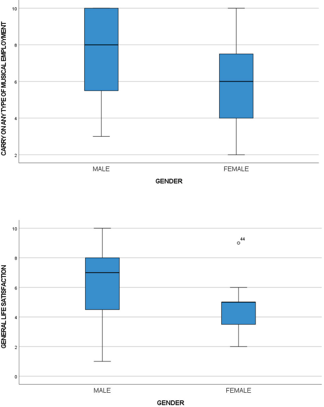
Figure 9.
Box plots of V5 (up) and V8 (down) by gender.
Table 7.
Results of inference (gender-V3, V6 and V7).
| Model 2 (music studies) | V3 (expectations on future income recovery) | V6 (expectations on own activity demand recovery) | V7 (expectations on live concerts' demand recovery) |
|---|---|---|---|
| Total No. | 55 | 55 | 55 |
| Mann-Whitney’s U | 245.500 | 200.000 | 218.500 |
| Wilcoxon’s W | 521.500 | 476.000 | 494.500 |
| Test statistic | 245.500 | 200.000 | 218.500 |
| Standard error | 57.947 | 58.099 | 58.128 |
| Standardised test statistic | −2.114 | −2.892 | −2.572 |
| Asymptotic sig. (bilateral test) | 0.035 | 0.004 | 0.010 |
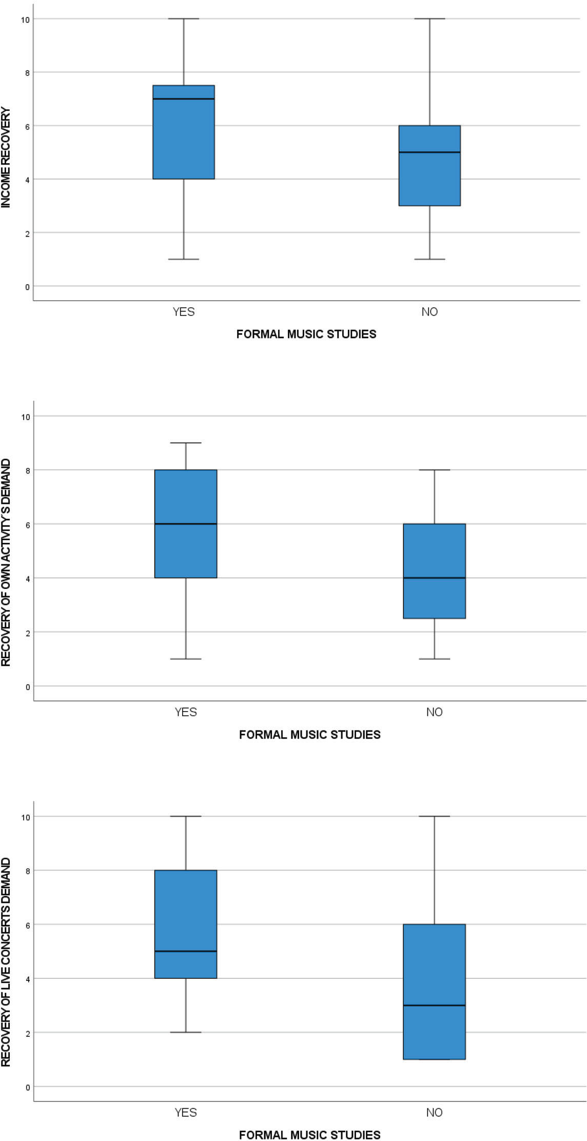
Figure 10.
Box plots of V3 (up), V6 (middle) and V7 (down) by music studies.
Table 8.
Results of inference (other job – V7).
| Model 3 (other job) | V7 (expectations recovery of the demand live concerts) |
|---|---|
| Total No. | 55 |
| Test statistic | 10.712a |
| Degrees of freedom | 3 |
| Asymptotic sig. (bilateral test) | 0.013 |
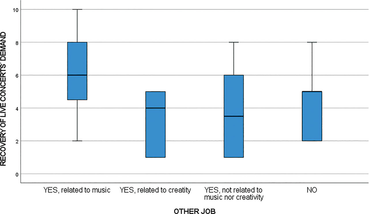
Figure 11.
Box plots of V7 by other job.
Table 9.
Results of inference (age, V4).
| Model 4 (age) | V4 (expectations regarding carrying on with own activity) |
|---|---|
| Total No. | 55 |
| Mann–Whitney’s U | 530.500 |
| Wilcoxon’s W | 1,058.500 |
| Test statistic | 530.837 |
| Standard error | 57.837 |
| Standardised test statistic | 2.810 |
| Asymptotic sig. (bilateral test) | 0.005 |
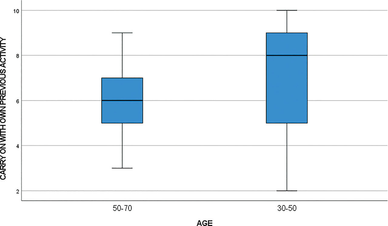
Figure 12.
Box plots of V4 by age.
Table 10.
Correlation rates (V1, V2 – V3–V8).
Table 11.
Results on inference tests.
| Independent variable | Hypothesis | Affected variable | Sig. level | |
|---|---|---|---|---|
| V1 | Impact of COVID-19 on activity | H8 | V3 | 0.046 |
| V2 | Impact of COVID-19 on income | H9 | V3 | 0.027 |
| H10 | V4 | 0.029 | ||
| H11 | V7 | 0.031 |
Table 12.
Results of inference (impact of COVID-19 on activity-V3).
| Model 4 (activity) | V3 (expectations on future income recovery) |
|---|---|
| Total No. | 55 |
| Test statistic | 8.001a |
| Degrees of freedom | 3 |
| Asymptotic sig. (bilateral test) | 0.046 |
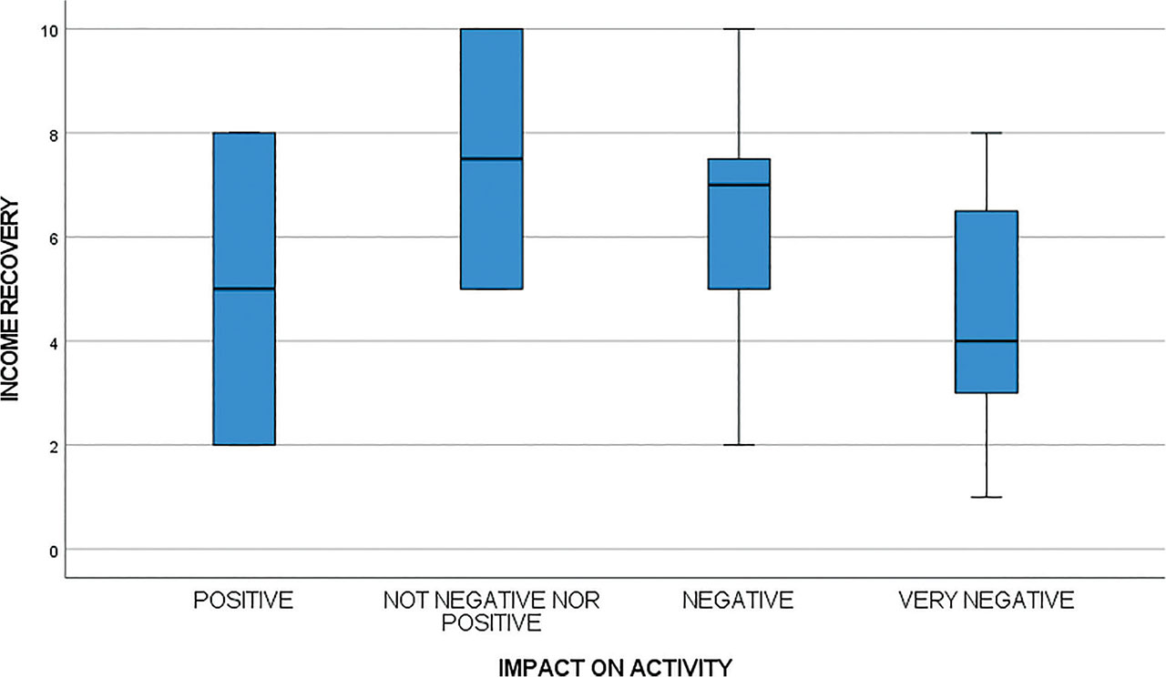
Figure 13.
Box plots of V3 by V1 (impact of COVID-19 on activity).
Table 13.
Results of inference (impact of COVID-19 on income-V3, V4, V7).
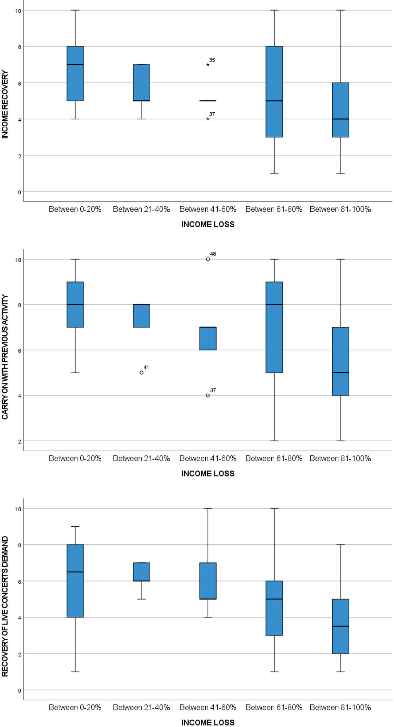
Figure 14.
Box plots of V3 (up), V4 (middle) and V7 (down) by V2.