
Introduction
Background and Motivation
In recent years, data-driven tactical analysis has advanced rapidly in team sports, including soccer (Fujii, 2025; Mgaya, Liu, & Zhang, 2021). While match analysis previously relied heavily on subjective expert knowledge, advancements in video analysis technology have enabled the objective evaluation of player behavior using tracking data (Dick & Brefeld, 2019; Forcher et al., 2022; Herold et al., 2019; Torres-Ronda et al., 2022). Furthermore, research efforts have expanded from individual player actions to the objective evaluation of the team’s tactical intentions (Bialkowski et al., 2016; Feuerhake, 2016; Lucey et al., 2021; Tenga et al., 2009). Within this domain, play phases, which capture the flow of a match in distinct tactical segments, are a crucial concept for understanding team intentions and structure (Hewitt et al., 2016).
The concept of play phases has evolved. The most fundamental classification has long been the binary division into attack and defense (Duarte et al., 2014). Alternative perspectives have emerged, such as the classification of soccer into three broad phases: attack, defense, and preparation or midfield play (Wade, 1996). Furthermore, it has been suggested that the game consists of four primary recurring phases, or moments: Established Attack, Defensive Transition, Established Defense, and Offensive Transition (Oliveira, 2004). This four phase framework is extensively utilized in coaching, and the expanded model (Hewitt et al., 2016)—which incorporates set pieces as a fifth distinct moment—is also now widely adopted. Beyond these four broad phases, more granular phases, such as build up or counter-attack, are also utilized in practical coaching to provide more detailed instructions (Barnerat et al., n.d.). Consequently, there is a growing demand for a universal automatic play phase recognition technology that can be understood and utilized by any team or broadcaster. If realized, such technology would significantly enhance the efficient evaluation, sharing, and coaching of team tactics by providing a standardized framework for analysis.
In response to this need, various approaches have been explored in existing research. Some studies have aimed to estimate the basic four phases (Kempe et al., 2014.; Merlin et al., 2020). Others have reported methods for recognizing more specific phases, such as counter-attack or counter-press (Bauer & Anzer, 2021; Fassmeyer et al., 2021; Kobayashi, Kawamura, & Suzuki, 2012; Kuroda et al., 2024; Sigari et al., 2015). Additionally, research classifying matches into several phases using unsupervised learning has also been reported (Decroos, Van Haaren, & Davis, 2018; Grunz, Memmert, & Perl, 2012; Michael et al., 2018; Wang et al., 2015). However, these studies have not yet established a truly universal automatic play phase recognition technology. A primary reason is that a general definition of play phases has not been widely disseminated; consequently, unified definitions have not been applied across these studies.
As a notable effort to bridge this gap, Bauer (2022) defined 11 tactical patterns within five game-states. These definitions were refined through a series of consultations with German Bundesliga professionals to ensure high practical applicability. While this framework provides a comprehensive overview, it is specifically designed to extract noteworthy tactical patterns by defining each phase individually.
Similarly, the International Federation of Association Football (FIFA) published a “phases of play” framework that defines nine major phases (Table A1 in the Appendix; FIFA, 2022). These definitions are rooted in the tactical understanding widely utilized in general coaching. Unlike Bauer’s extractive approach, the FIFA model aims to categorize every possible match situation into its respective play phases, making it more structurally suited for a continuous automated recognition task. By targeting these FIFA-defined phases for estimation, this study ensures a general-purpose understanding of the results and contributes to the establishment of standardized tactical recognition technology.
Challenge
Specific moments in a soccer match cannot always be clearly classified into a single play phase, even when applying standardized definitions such as those provided by FIFA. When experts analyze a game, they may perceive a situation as having multiple possible interpretations or as an ambiguous phase where several tactical intentions coexist. This difficulty in achieving a consistent consensus is underscored by Bauer and Anzer (2021), who reported that even when three analysts annotated a specific tactical pattern, the pairwise inter-labeler accuracy remained at 82.01%. This ambiguity arises from the complex nature of soccer, where each of the 11 players possesses their own perception of the match situation. The collective team phase then emerges from the integration of these diverse individual perspectives.
This complexity suggests that play phase recognition is a probabilistic phenomenon rather than a deterministic, single-label event. Directly estimating probability distributions from spatiotemporal data yields a richer tactical context than traditional classification. From a practical perspective, this granular representation benefits both media and professional analysis. For sports broadcasting, it facilitates automated live commentary by providing nuanced linguistic inputs essential for natural language generation. For professional analysts, it enables rigorous investigations into how team formations and expected goals (xG) fluctuate in response to shifting match contexts.
Despite this potential, much of the existing research on automatic recognition formulates the problem as a classification task that assigns a single label to each moment (Fernandez-Navarro et al., 2016; Niu, Gao, & Tian, 2012; Suzuki et al., 2019). While some studies utilize models that output probabilities, they typically convert these results into a single category using a fixed threshold for classification purposes (Bauer et al., 2023; Kamiya et al., 2017). To the best of our knowledge, few studies have explicitly argued for the importance of representing play phases as a continuous probability distribution to preserve tactical nuance.
A primary obstacle is that representing a reliable ground truth for such a probability distribution remains a significant challenge. In response, we explore a method to represent this probability distribution by leveraging diverse opinions from multiple analysts.
Proposed Approach and Contributions
This study proposes a method to estimate the probability distributions of play phases An overview of our proposed approach is illustrated in Figure 1.
As a foundation for this approach, we represent a probability distribution of play phases by aggregating annotations from multiple analysts, as depicted in Figure 1(a). First, multiple analysts independently review the match footage and assign a single play phase according to the official FIFA definitions at every moment. This probability distribution is then formed by aggregating these individual assignments.
Next, as shown in Figure 1(b), we develop a deep learning model to estimate the probability distribution of play phases. This model is trained using the probability distributions obtained from the annotation as ground-truth labels. A key feature of this model is its ability to probabilistically estimate the play phases (e.g., “30% counter-attack, 70% build up”) for a given match scene. The model input uses trajectory data for all 22 players and the ball, extracted from video footage. This is based on the hypothesis that the tactical intentions of players and teams manifest as trajectories on the pitch.
The main contributions of this paper are as follows:
We formulate a new task that models, as a probability distribution, the inherent ambiguity in play phases estimation that arises from applying the FIFA-defined phases of play.
We propose a novel method to represent this probability distribution by aggregating diverse perceptions from multiple analysts.
We designed a deep learning model to estimate this probability distribution from the constructed dataset and demonstrated its effectiveness.
We have made the dataset, pre-trained models, and Python modules publicly available to facilitate further research and ensure the reproducibility of our findings.
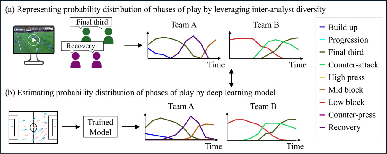
Figure 1:
Overview of this study. This study proposes a method to estimate the probability distribution of FIFA-defined phases of play. First, as depicted in (a), we represent the probability distribution of play phases by leveraging inter-analyst diversity. Subsequently, as shown in (b), this represented probability distribution serves as the ground truth for training a deep learning model to estimate the probability distribution of phases.
Proposed Method
Representing Probability Distributions of Play Phases by Leveraging Inter-Analyst Diversity
This section describes the process of representing the probability distributions of play phases by leveraging the diversity among analysts.
Definition of Play Phases
In this study, analysts annotated match footage according to the definitions of phases of play provided by FIFA (FIFA, 2022). FIFA defines 16 phases of play that a team can be in at any given time, among which 9 are considered principal phases. Each of these 9 phases is described by a definition ranging from two to ten lines in English as shown in Table 1. This study targets these 9 principal phases, as shown in Table 1. We denote the set of these target phases as 𝒫, and each element as pi ∈ 𝒫(i = 1, … , 9) using the symbols p1 to p9 as shown in Table 1.
Representation of Probability Distributions
Annotation by a Single Analyst: A single analyst annotates a team’s play phase as either one of the phases pi ∈ 𝒫 or as ɛ, which signifies “not applicable.” We define the complete set of labels, including ɛ, as 𝒬 = 𝒫 ∪ {ϵ}, with each element qj ∈ 𝒬 (j = 1, … , 10). The annotation by analyst k ∈ {1, … , N} for team l ∈ {1,2} at time t is formulated as a probability distribution Pk,l,t, defined as a one-hot vector in Equation (1).
Here, Pk,l,t(qj) takes a value of 1 if analyst k annotates the phase of team l at time t as qj, and 0 otherwise. The sum of the elements in Pk,l,t satisfies .
Aggregation of Multi-Analyst Annotations: Rather than employing a majority vote to produce a single one-hot label, we treat the annotations from N analysts as a probability distribution that captures the diversity of expert opinions. The probability distribution of play phases for team l at time t, TPl,t, is defined in Equation (2).
Each element TPl,t(qj) is defined in Equation (3) as the proportion of the N analysts who annotated the phase of team l at time t as qj.
While the value of TPl,t(qj) is restricted to discrete increments of 1⁄N within the range [0, 1], it functions as a quasi-continuous representation of collective analyst judgment. This distribution ranges from 0 (unanimous disagreement) to 1 (unanimous agreement) and satisfies the constraint .
In conventional approaches that do not consider diversity, the team’s play phases are represented as a one-hot vector , as shown in Equation (4).
Each element is defined by Equation (5).
Following the precedent of prior studies using two or three analysts, a play phase is typically assigned only when a consensus is reached by at least two individuals. Consistent with this principle, our formulation defines a majority as agreement from more than half of the analysts. In the event of a tie-break where no single phase achieves a strict majority, the sequence is not assigned to any specific tactical category.
Annotation Datasets
This study uses the SoccerTrack v2 dataset (Scott et al., 2025). This dataset comprises match footage, tracking data, and event data from 10 amateur-level matches, primarily from the University of Tsukuba. The match footage was captured using Bepro’s camera system. This system generates a seamless panoramic video overlooking the entire pitch by automatically stitching footage from three cameras installed on the sidelines.
Due to limited resources regarding the number of analysts and available annotation time, we strategically extracted in-play sequences from the 10 matches, totaling approximately 180 minutes. The in-play sequences range from 30 seconds to 6 minutes. During selection, we prioritized scenes with frequent transitions, specifically ensuring that transitions account for nearly half of each in-play sequence. This selection strategy serves two primary purposes. First, it balances the dataset for model training; while defensive and offensive phases like build up often exceed 30% of match time, transition phases such as counter-attack typically account for less than 5% (FIFA, 2022). Second, it incorporates inherent ambiguity into the dataset. Unlike the more distinct offensive and defensive phases, transition phases are harder to define and more prone to diverse interpretations among experts, providing a more robust foundation for probabilistic modeling.
Annotation Process
The annotation is conducted by a total of 16 analysts, comprising 14 members of the University of Tsukuba Football Club’s analysis team and 2 individuals with equivalent soccer and analysis experience. To manage the workload, the 180 minutes of match footage are divided into four sets of approximately 45 minutes each. Each set is assigned to a group of four analysts, ensuring that every moment in the dataset is independently annotated by four individuals (N = 4 in Equation (2).
While existing studies typically rely on a cross-check between only two or three independent labelers (Bauer et al., 2023; Bauer & Anzer, 2021; Chawla et al., 2017), our framework employs four independent analysts per set. This multi-analyst approach provides a more robust cross-check and significantly higher reliability in representing the ground truth. To ensure the integrity of this independent evaluation, all analysts work individually without access to the annotations of others.
The task is conducted using a dedicated application provided by Bepro, as shown in the interface screenshot in Figure A1. The software allows the use of an AI-powered video that automatically tracks and zooms in on the ball or specific players. The task is performed via keyboard operations, with keys ‘0’ through ‘9’ assigned to each element of 𝒬 (the 9 phases plus ɛ). When an analyst judges that the focused team has transitioned to a specific phase, they press the corresponding key. To maintain consistency with international standards, analysts are permitted to refer to a paper copy of the FIFA phase definitions at any time during the process. Each analyst first focuses on one team for the 45-minute video and then repeats the process for the opposing team, resulting in approximately 90 minutes of work per analyst.
Estimating Probability Distributions of Play Phases by Deep Learning Model
This section describes the process of developing the deep learning model to estimate probability distributions of play phases.
Problem Formulation
Input Representation: This study uses the trajectory data of 22 players and the ball included in the SoccerTrack v2 dataset as input to the deep learning models. First, we define the state variable at time t. The set of positions for the ball and all players from both teams, denoted by Xt, is defined in Equation (4).
Here, represent the 2D on-pitch coordinates of the ball, the a-th player of team 1, and the b-th player of team 2, respectively.
The time-series sequence 𝒳T, which serves as the model input, is defined as the sequence of states collected over a duration of 2L seconds (L seconds before and after the center time T), as shown in Equation (5).
In this study, we set the window duration to L = 10 s (10 s before and 10 s after the center time) and the sampling frequency to fs = 5 Hz (Δt = 0.2 s). Consequently, the length of each input sequence is W = 2 × L × fs = 100 frames.
Target Representation: The target probability distribution of play phases for team l at time T, denoted as Yl,T, is defined as a 9-dimensional vector whose elements represent the probabilities of the 9 phases, as shown in Equation (6).
Here, yl,T(pi) denotes the probability that team l is in phase pi at time T. As described earlier, we aggregate the annotations from N = 4 analysts to construct the ground-truth label. Consequently, each element of the target vector takes one of the discrete values listed in Equation (7).
Learning Objective: The deep learning model f is trained as a regression function, f(𝒳T) = Yl,T, that predicts the probability distribution Yl,T from the input sequence 𝒳T.
For the ablation study, we additionally consider two alternative ground-truth labels for comparison:
Training Dataset
We utilize spatiotemporal tracking data from the SoccerTrack v2 dataset. These trajectories, representing the ball and all 22 players, are extracted at 25 fps using Bepro’s proprietary optical tracking system from full-pitch panoramic videos. The reliability of this technology is underscored by its FIFA Quality Certification for Electronic Performance and Tracking Systems (EPTS) (BEPRO, 2022). In official FIFA validation tests, Bepro’s fixed and portable camera systems achieved performance ratings that significantly exceed industry standards for both positional and velocity-based metrics. This high precision is maintained through a human-in-the-loop validation process and systematic data cleaning, ensuring that the trajectories meet professional-grade standards for tactical analysis across diverse match environments (BEPRO Dev Team, 2022). By utilizing these FIFA-certified commercial datasets, we aim to ensure that our proposed model is compatible with the data formats and accuracy levels currently prevalent in professional football coaching and analysis.
Prior to dataset construction, two specific in-play segments are set aside for qualitative evaluation to ensure the model is tested on unseen, continuous match scenarios. From the 180 minutes of annotated match footage, we extract training sequences using a sliding window approach. Specifically, for each in-play segment ranging from 30 s to 6 min, we generate 20-s input sequences by sliding the center time T in 0.2-s increments. To ensure temporal context, windows start 10 s after the beginning and end 10 s before the conclusion of each segment. This process yields a total of 50,553 unique sequence-target pairs.
To leverage the model’s design for single-team estimation and increase the dataset’s volume, we apply point-symmetry augmentation relative to the pitch origin. For each annotated sequence, we construct two separate training samples—one for each team. For the second team’s sample, all coordinates are flipped and normalized so that the attacking direction remains consistent from the model’s perspective. This effectively doubles the dataset size to 101,106 samples.
The augmented dataset is partitioned into training, validation, and test sets on a per-segment basis to prevent data leakage. We utilize an optimization algorithm that assigns each in-play segment based on its internal phase scores. This approach minimizes the statistical discrepancy of play phases across the three sets by minimizing a quadratic error function, as detailed in the Segment Assignment Optimization section of the Appendix. This ensures that each set maintains a balanced representation of tactical patterns. Consequently, this segment-wise partitioning results in an approximate distribution of 80%, 10%, and 10% for the respective datasets relative to the total phase occurrences.
Training Setup
We employ the Huber Loss as the objective function for training. Huber Loss behaves quadratically like the L2 loss for small errors and linearly like the L1 loss for large errors. This characteristic allows it to achieve both stability in training and robustness to outliers, making it well-suited for our task of regressing continuous labels.
The batch size is unified to 128 for all models. We adopt the AdamW optimizer (Loshchilov & Hutter, 2017) with a weight decay of 10−5 for all experiments. To further prevent overfitting, we set a dropout rate of 0.1 across all models. The maximum number of training epochs is set to 300, and Early Stopping is applied to all models. Specifically, training terminates if the validation loss does not improve for 20 consecutive epochs, and the model weights from the epoch with the minimum validation loss are adopted. To ensure convergence to a finer local optimum, the learning rate is halved if the validation loss fails to improve for 10 consecutive epochs. This adjustment allows the model to perform more precise weight updates when the learning process reaches a plateau. The initial learning rate for each model is selected from a candidate set of {10−3, 5 × 10⁻⁴, 10−4} based on the best performance on the validation dataset. Furthermore, to ensure a fair comparison, we individually adjust the hidden dimensions and architectural parameters of each model so that their total number of parameters is approximately equal to 140k.
Model Architecture
In this study, we design and comparatively evaluate four deep learning models with different characteristics for the task of play phases estimation. For all models, the input consists of the 20 coordinates of the ball and all 22 players. In the Transformer and Baller2vec models, these are structured as a matrix , where W is the sequence length and D is the feature dimension. The feature dimension D is constructed by concatenating the 20 coordinates of the ball, the 20 coordinates of all 11 players from team 1, and the 20 coordinates of all 11 players from team 2, in that specific order (D = 23 × 2 = 46). Within each team, players are ordered by their tactical roles (e.g., GK, 0F, MF, FW). In contrast, the Graph Convolutional Network (GCN)+Transformer and Graph Attention Network (GAT)+Transformer models treat the input as a graph, denoted as 𝒳T in Equation (7). The graph structure is defined by a static adjacency matrix where edges exist between teammates and between the ball and all players, while no edges are defined between opposing players.
Transformer: We implement a Transformer encoder (Vaswani et al., 2017), to capture temporal dependencies. The input is projected onto a dmodel-dimensional latent space via a linear embedding layer, followed by the addition of sinusoidal positional encodings. The encoder consists of L = 3 layers, each configured with M = 4 attention heads, a dmodel of 60, and a feed-forward dimension of 4 × dmodel. To aggregate temporal information, the latent representation of the final time step is extracted and passed through a fully connected layer to produce the 9-dimensional output.
Baller2vec: This model extends the Transformer by incorporating agent-wise attention (Alcorn & Nguyen, 2021). The 20 coordinates are first concatenated with player I0 embeddings and projected through a multi-layer perceptron (MLP) to a dmodel-dimensional space. At each time step, a learnable CLS token is appended to the set of player and ball embeddings. Unlike the baseline Transformer, baller2vec captures spatiotemporal dependencies by applying self-attention across the unified sequence of all agents over time, governed by a custom self-attention mask to maintain temporal causality. To manage the computational cost of this multi-dimensional attention, the sequence length is downsampled from 100 to 20 frames. The model uses L = 3 layers with M = 4 heads and dmodel = 64. The final probability distribution is produced by a linear classifier applied to the CLS token representation from the final time step.
GCN+Transformer: This architecture employs a 2-layer GCN (Kipf & Welling, 2016) for spatial feature extraction, followed by a Transformer for temporal integration. At each time step, the GCN aggregates features from 2-hop neighboring nodes based on the adjacency matrix 𝒳T. This two-layer configuration is chosen to capture higher-order tactical relationships, such as third-man positioning, while avoiding the over-smoothing common in deeper graph networks. To transform the spatial node embeddings into a format suitable for temporal analysis, we utilize a set-attention mechanism. A single learnable query vector performs multi-head attention over the GCN-derived node embeddings to pool spatial information from the 22 players and the ball into a compact representation. The resulting feature vectors have a dimension dmodel of 64, which is the product of the hidden dimension and the number of queries. These vectors form a time-series sequence for a Transformer encoder with L = 3 layers, M = 4 heads, and a feed-forward dimension of 2 × dmodel. Finally, the latent representation of the last time step passes through a fully connected layer to produce the play phase probability distribution.
GAT+Transformer: This model replaces the GCN with a 2-layer GAT (Veličković et al., 2017) to enable more adaptive spatial feature extraction. The GAT operates on the same graph structure 𝒳T but dynamically learns attention weights to prioritize critical tactical interactions, such as those between a ball carrier and support players. The first GAT layer employs M = 4 attention heads followed by an ELU activation, while the second layer aggregates these features into a single-head representation. Similar to the GCN-based model, a single learnable query vector is used via a set-attention mechanism to pool the resulting node embeddings into a dmodel-dimensional frame representation. This spatial feature, with a dimension of 64, is then processed by a Transformer encoder with L = 3 layers, M = 4 heads, and a feed-forward dimension of 2 × dmodel. Finally, the latent representation of the last time step is passed through a fully connected layer to produce the output.
Experimental Setup and Evaluation Metrics
Quantitative Evaluation of Dataset Characteristics
We assess the characteristics of the constructed probability distribution dataset, focusing on the diversity and reliability among analysts.
First, we quantify the extent of diversity through two complementary approaches. We analyze the occurrence ratio of annotation patterns (e.g., “all four analysts agree”) to grasp the global distribution of consensus across the total match duration. To further examine phase-specific characteristics, we also visualize the consensus levels for each individual play phase. This dual-metric approach allows us to distinguish between the overall dataset diversity and the inherent ambiguity within specific play phase.
Second, we introduce a pairwise confusion matrix to visualize the tendencies of analyst disagreement. To account for all perspectives, we calculate confusion matrices for every possible pair of the four analysts and aggregate the results. The matrix illustrates the probability that another analyst selected phase pj given that a specific analyst selected phase pi. This helps identify which specific phases are most prone to perceptual diversity.
Third, we evaluate inter-analyst agreement using Krippendorff’s α (Krippendorff, 2011). While simple agreement metrics like Cohen’s Kappa are commonly used, they are insufficient for this study as we intentionally incorporate diverse expert interpretations. By incorporating a semantic distance metric into the α calculation, we can distinguish whether the observed diversity stems from unreliable random labeling or from meaningful variations within semantically related play phases.
We define this semantic distance based on a three-level hierarchical structure of play phases: ball possession (Level 1), phase stability (Level 2), and specific tactical categories or intensity thresholds (Level 3). In this hierarchy, the 9 play phases are categorized into four high-level phases as follows: “Offensive” includes Build-up, Progression, and Final third; “Transition to Offense” consists of Counter-attack; “Defensive” comprises High press, Mid block, and Low block; and “Transition to Defense” includes Counter-press and Recovery. The distances are assigned according to the severity of the disagreement:
Distance 0.00 (Agreement): Identical play phases.
Distance 0.25 (Level 3 Error): Disagreements between sub-categories within the same high-level four phases (e.g., build up vs. progression). This also applies to disagreements involving the “No label” (ɛ) category, as these typically reflect subjective differences in intensity thresholds—whether a phase is distinct enough to be labeled—rather than a structural misunderstanding of the game.
Distance 0.50 (Level 2 Error): Disagreements regarding phase stability (e.g., offensive vs. transition to offense) while maintaining the same possession context. This reflects the inherent temporal ambiguity in identifying the exact moment of a turnover.
Distance 1.00 (Level 1 Error): Disagreements in ball possession (e.g., offensive vs. defensive). This represents a fundamental misinterpretation of the tactical situation and is thus assigned the maximum penalty.
The values 0.25, 0.50, and 1.00 were chosen to reflect an exponential scaling of disagreement severity. This ensures that fundamental structural errors (Level 1) are penalized significantly more than minor interpretative variations (Level 3), providing a more robust measure of tactical reliability than linear weighting. The specific distances between the four high-level phases are summarized in Table 2.
Quantitative Evaluation of Model Performance
To evaluate the necessity of the proposed spatial and temporal architectures, we compare our models against two reference baselines. The first is Mean Prediction, a non-learning baseline that consistently outputs the average probability distribution of the training set. This baseline represents the performance achievable by merely accounting for the dataset’s class imbalance. The second is an MLP, a simple deep learning baseline that processes input features as flattened vectors. To ensure a fair comparison, the MLP is configured to have approximately 140k parameters, consistent with the other models in this study. This baseline clarifies whether complex architectures, such as GNNs and Transformers, are necessary for capturing tactical patterns beyond simple mappings from coordinates to labels.
Our task is formulated as a regression problem to predict the probability distributions of play phases. Mean Absolute Error (MAE) is calculated by first averaging the absolute differences between the predicted probabilities and the ground-truth labels across all sequences in the test set for each play phase. The final MAE is then determined by taking the average of these values across all nine play phases. Similarly, Root Mean Square Error (RMSE) is computed by averaging the squared differences for each phase over all test sequences, taking the square root, and then calculating the mean across all phases. By applying this two-step averaging process, RMSE penalizes larger prediction discrepancies more heavily than MAE while providing a balanced assessment of performance across all tactical categories.
Furthermore, we evaluate the model using Top-1 Accuracy (Top-1 Acc) and Top-3 Accuracy (Top-3 Acc). Top-1 Acc represents the percentage of samples where the model’s most probable phase matches the ground-truth’s primary phase. Similarly, Top-3 Acc measures the frequency with which the ground-truth’s primary phase is included within the model’s three most probable phases. These accuracy metrics are calculated exclusively for the subset of samples where the highest probability in the ground truth is greater than or equal to 0.75, ensuring that evaluation is focused on instances with high analyst agreement. The Top-1 Accuracy is defined as follows:
where S denotes the subset of samples with high analyst agreement, and 𝟙[·] is the indicator function.All reported overall metrics are calculated as the macro-average of the values obtained for each play phase, ensuring that the model’s performance is evaluated equitably across all play phases regardless of their frequency in the dataset.
After comparing the aggregated metrics to identify the most effective architecture, we perform a detailed analysis of the results per play phase using the best-performing model. This granular evaluation allows us to investigate the specific predictive difficulty associated with each play phase.
Qualitative Evaluation
We conduct two types of qualitative evaluation to assess different aspects of the model’s performance.
First, to visually inspect how well the trained model replicates the ground truth, we use the sequences previously set aside for visualization. For these sequences, we visualize the probability distribution of play phases as represented by inter-analyst diversity (i.e., the ground-truth distribution) and compare it side by side with the probability distribution predicted by the trained deep learning model. This qualitative analysis focuses on a single team to closely examine the model’s ability to estimate the complex, ambiguous states defined by the analysts.
Second, to evaluate the model’s generalization performance, particularly its ability to adapt to Out-of-Distribution data different from our amateur training data, we use professional match data from La Liga acquired from Skillcorner as an external test set. The reliability of SkillCorner’s tracking technology is validated by its FIFA Basic certification under the Quality Programme for EPTS, ensuring professional-grade accuracy in broadcast-based data (May, 2024). We qualitatively evaluate the prediction results on approximately 30 seconds of data from the Real Madrid vs. FC Barcelona match (23/24 season, April 21, 2024).
Ablation Study
We conduct two ablation studies to verify the effectiveness of the components of our proposed methodology.
Probabilistic Labels vs. Deterministic Labels: This study validates the effectiveness of training on continuous probability distributions as defined in Eq.(9) rather than conventional discrete labels as defined in Eq. Error! Reference source not found.). We compare the performance of our approach against the same model architectures trained using deterministic labels derived from a majority vote as defined in Eq. (4).
Single-Team Learning vs. Dual-Team Learning: We investigate the impact of incorporating the opponent’s play phase as simultaneous contextual information. For this purpose, we compare our proposed model, which predicts a 9-dimensional label for a single target team, against an alternative model that simultaneously predicts 18-dimensional labels covering both teams as shown in Eq. Error! Reference source not found.). This comparison clarifies whether multi-team prediction improves the estimation accuracy of the target team’s tactical phases.
Results
Quantitative Results of Dataset Characteristics
The occurrence ratio of annotation patterns across the entire dataset is shown in Figure 2. We categorized the patterns into four types: (1) all four analysts agreed; (2) three analysts agreed; (3) diversity-prominent patterns (two analysts agreed or all disagreed); and (4) consensus on “No label.” The analysis reveals that while agreement-leaning patterns (1 and 2) account for over 50% of the total duration, diversity-prominent patterns (3) remain significant at approximately 40%.
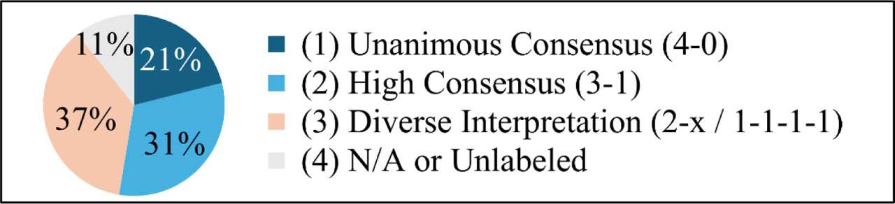
Figure 2:
Global proportion of annotation patterns. The patterns are classified based on the level of consensus relative to the total match duration to provide an overview of dataset diversity without temporal overlaps.
The detailed content of this diversity is further broken down by play phase in Figure 3. This visualization confirms that for every category, we obtain a rich probability distribution derived from the four analysts’ independent perspectives. Relatively static play phases, such as build up and mid block, show a higher proportion of consensus with three or more analysts in agreement. In contrast, dynamically occurring phases with shorter durations, such as counter-attack and counter-press, exhibit an extremely small proportion of full consensus among all four analysts.
In Figure 3, the proportions for “1 Analyst Only” and “2 Analysts Agree” appear more prominent than in the global aggregate. This is because when analysts disagree, their labels often overlap across different phases for the same time step, effectively increasing the counts in these lower-consensus categories.
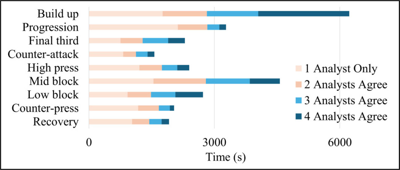
Figure 3:
Distribution of consensus levels across play phases. The vertical axis lists the play phases, and the horizontal axis shows the total annotated time in seconds. The legend classifies the duration based on the number of analysts in agreement.
Next, we analyze the content of this diversity in detail using the pairwise confusion matrix in Table 3. The results show that relatively static phases (Build up, Final third, Low block) have strong diagonal components, indicating a high tendency for analyst agreement. Conversely, transition-related phases (Counter-attack, Counter-press, Recovery) show weaker diagonal components, confirming that perceptions are more likely to be dispersed. Notably, progression was often perceived as build up by other analysts, suggesting it is an ambiguous phase prone to diversity.
Table 3:
Aggregated pairwise confusion matrix across all four analysts. Each cell (i, j) represents the frequency with which an analyst assigned phase pj while another analyst assigned phase pi to the same frame, normalized by the total number of pairwise comparisons.
| Build up | Progression | Final third | Counter-attack | High press | Mid block | Low block | Counter-press | Recovery | No label | |
|---|---|---|---|---|---|---|---|---|---|---|
| Build up | 0.71 | 0.10 | 0.03 | 0.01 | 0.01 | 0.01 | 0.01 | 0.02 | 0.01 | 0.09 |
| Progression | 0.39 | 0.32 | 0.08 | 0.04 | 0.01 | 0.01 | 0.01 | 0.03 | 0.01 | 0.11 |
| Final third | 0.06 | 0.11 | 0.66 | 0.06 | 0.00 | 0.01 | 0.00 | 0.04 | 0.01 | 0.06 |
| Counter-attack | 0.05 | 0.09 | 0.11 | 0.45 | 0.03 | 0.04 | 0.06 | 0.04 | 0.01 | 0.11 |
| High press | 0.02 | 0.01 | 0.00 | 0.02 | 0.53 | 0.20 | 0.04 | 0.05 | 0.04 | 0.08 |
| Mid block | 0.02 | 0.01 | 0.00 | 0.01 | 0.10 | 0.58 | 0.11 | 0.02 | 0.04 | 0.11 |
| Low block | 0.02 | 0.00 | 0.00 | 0.02 | 0.01 | 0.07 | 0.70 | 0.02 | 0.09 | 0.07 |
| Counter-press | 0.08 | 0.05 | 0.07 | 0.02 | 0.11 | 0.04 | 0.04 | 0.36 | 0.12 | 0.12 |
| Recovery | 0.04 | 0.01 | 0.02 | 0.01 | 0.04 | 0.08 | 0.12 | 0.08 | 0.48 | 0.12 |
| No label | 0.10 | 0.04 | 0.04 | 0.02 | 0.04 | 0.06 | 0.05 | 0.05 | 0.03 | 0.59 |
Finally, we evaluate the inter-analyst agreement using Krippendorff’s α. The α calculated with a simple nominal metric (categorical agreement) was 0.52. In contrast, when weighted by the semantic distance defined in Table 2, the α value significantly increased to 0.68. This improvement from 0.52 to 0.68 quantitatively demonstrates that the analysts’ annotations were not randomly dispersed. Instead, they maintained semantic consistency based on the four phases model while making diverse interpretations within those phases.
Quantitative Results of Model Performance
We evaluate the estimation accuracy of the four models. Each model, trained according to the setup described previously, was used to perform estimation on the test data, and the results were evaluated using MAE, RMSE, Top-1 Acc, and Top-3 Acc. The results are shown in Table 4. Among the four models, GAT+Transformer demonstrated the best performance across all metrics. Additionally, baller2vec and GCN+Transformer outperformed the other models, likely because baller2vec utilizes inter-player attention to handle sequences regardless of player ordering, while graph-based methods capture spatial relationships by treating player positions as permutation-invariant structures.
Table 4:
Model performance evaluation.
| Model | MAE | RMSE | Top-1 Acc (%) | Top-3 Acc (%) |
|---|---|---|---|---|
| Mean Prediction | 0.14 | 0.21 | 11 | 33 |
| MLP | 0.08 | 0.20 | 22 | 49 |
| Transformer | 0.08 | 0.21 | 22 | 51 |
| baller2vec | 0.06 | 0.16 | 48 | 68 |
| GCN+Transformer | 0.07 | 0.18 | 39 | 71 |
| GAT+Transformer | 0.06 | 0.16 | 49 | 80 |
To further investigate the characteristics of the play phase estimation, we analyze the performance of the GAT+Transformer model, which achieved the highest overall accuracy, for each individual phase. Table 4 presents the MAE, RMSE, Top-1 Acc, and Top-3 Acc for the 9 play phases.
The results reveal a discrepancy between regression metrics and classification accuracy. Dominant phases like “Build up” and “Mid block” exhibit higher MAE and RMSE due to their frequent occurrence and high probability scores (near 1.0), which increase absolute error magnitude. Nevertheless, their exceptionally high Top-1 Accuracy indicates that the model reliably identifies them as the primary phase. Conversely, infrequent phases such as “Counter-attack” show lower MAE and RMSE but significantly poorer Top-1 Accuracy. This is primarily driven by the class imbalance shown in Figure 3, where “Build up” and “Mid block” durations far exceed others, making it difficult for the model to prioritize rare phases. Additionally, these phases often involve higher analyst disagreement, characterized by lower probability scores (0.25 and 0.50) rather than definitive labels. This inherent ambiguity further complicates achieving high confidence in Top-1 predictions.
Table 5:
Estimation performance per play phase for the GAT+Transformer model.
| Phase | MAE | RMSE | Top-1 Acc (%) | Top-3 Acc (%) |
|---|---|---|---|---|
| Build up | 0.11 | 0.21 | 91 | 98 |
| Progression | 0.06 | 0.13 | 21 | 95 |
| Final third | 0.05 | 0.14 | 77 | 96 |
| Counter-attack | 0.05 | 0.18 | 0 | 25 |
| High press | 0.05 | 0.15 | 57 | 99 |
| Mid block | 0.09 | 0.19 | 94 | 100 |
| Low block | 0.05 | 0.14 | 88 | 96 |
| Counter-press | 0.04 | 0.14 | 0 | 30 |
| Recovery | 0.05 | 0.17 | 12 | 78 |
Qualitative Analysis
For the qualitative evaluation, we performed inference on two representative sequences using the GAT+Transformer model, which achieved the highest accuracy in our quantitative assessment. Figure 4 shows the estimation results of the probability distribution of play phases for a specific team in a sample sequence. The upper graph displays the probability distribution represented by leveraging the inter-analyst diversity, while the lower graph shows the results predicted by the trained model. As visually evident in Figure 4, the model accurately identifies sustained phases such as “High Press” and “Mid Block,” showing high alignment with the ground-truth probabilities. However, the model encounters difficulties in estimating transition phases, such as “Counter-attack” and “Recovery.” As discussed in the “Quantitative Results of Model Performance” section, the lower accuracy in these phases stems from the limited sample size in the dataset and the inherent ambiguity of transition moments, which often lead to low inter-analyst agreement. This qualitative observation reinforces the challenge of capturing transitions that lack distinct, long-term spatial patterns.
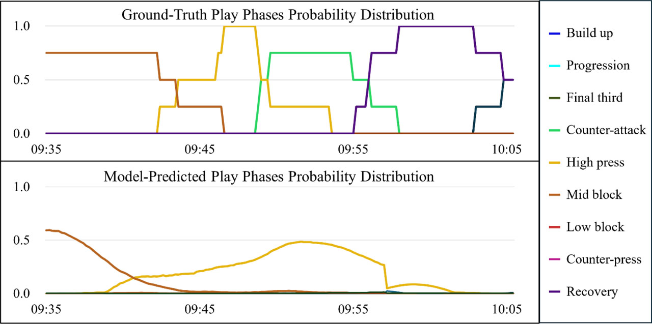
Figure 4:
Qualitative comparison of the probability distribution of play phases for a sample sequence. The upper graph shows the ground-truth distribution, aggregated from inter-analyst diversity. The lower graph shows the corresponding probability distribution predicted by the trained model.
Figure 5 shows the estimation results of the trained model on a La Liga match. The estimation results were acquired at 5 fps and concatenated to visualize the time-series estimations for each play phase. From this visualization, the transitions between offensive and defensive phases are intuitively identifiable, reflecting the dynamic nature of the match. Nevertheless, it should be noted that certain transition phases might be underrepresented or missing in the predictions where they are tactically expected. This discrepancy likely arises from the aforementioned difficulty in classifying brief transition events, suggesting that while the model captures the overall flow of the game, further refinement is needed to resolve rapid tactical shifts.
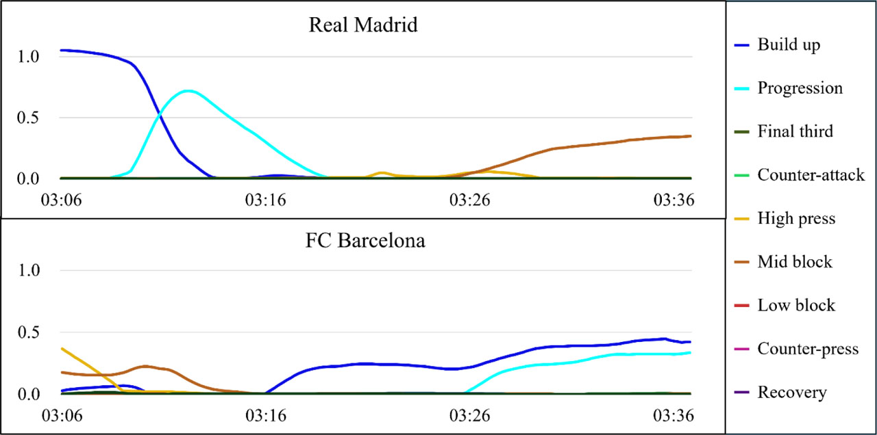
Figure 5:
Qualitative evaluation using a La Liga match. The upper graph shows the probability distribution of play phases for Real Madrid, while the lower graph shows the same for FC Barcelona.
Ablation Study
We conduct two ablation studies using the GAT+Transformer model, which achieved the highest quantitative accuracy, to verify the effectiveness of the components of our proposed method.
Probabilistic Labels vs. Deterministic Labels: Table 6 compares the model performance when trained on probabilistic labels versus deterministic labels. The results demonstrate that the model trained with probabilistic labels outperforms the deterministic counterpart across all evaluated metrics. This performance gap can be attributed to the inherent characteristics of the dataset. Our dataset contains numerous sequences where tactical interpretations vary among analysts, making it difficult for the model to converge when forced to learn from discrete, deterministic labels.
However, it is also possible that the observed performance drop stems from an imbalance in the dataset distribution rather than the labeling method alone. As illustrated in Figure 3, sequences with probability values of 0.25 or 0.50 are significantly more frequent than those with 0.75 or 1.00. Consequently, in the discrete labeling approach, the number of positive labels representing 1 is substantially lower than those representing 0, which may lead to insufficient training for specific tactical categories.
Table 6:
Performance comparison between models trained with continuous probabilistic labels and discrete deterministic labels.
| Label | MAE | RMSE | Top-1 Acc (%) |
|---|---|---|---|
| Probabi1istic Labe1s | 0.06 | 0.16 | 49 |
| Deterministic Labe1s | 0.08 | 0.21 | 28 |
Single-Team Learning vs. Dual-Team Learning: Table 7 shows the results. This comparison indicated that training the model to predict only the label for a single team (9 dimensions) resulted in better accuracy than predicting the labels for both teams simultaneously (18 dimensions). While it was expected that simultaneously learning the opponent’s play phases would allow the model to acquire a richer tactical context, it is suggested that, under this experimental setup, the increased task complexity accompanying the higher-dimensional output may have hindered the model’s learning.
Discussion
Several points warrant further discussion regarding the methodology and results of this study, categorized into the effectiveness and limitations of our annotation framework and the factors influencing model estimation performance.
Framework Effectiveness and Annotation Characteristics
The core contribution of this study is the proposal of a framework that represents play-phase probability distributions by leveraging the diverse perspectives of multiple analysts. As demonstrated in Figures 2 and 3, capturing these varied interpretations effectively quantifies the tactical uncertainty inherent in soccer. The high reliability and consistency of these generated distributions are quantitatively supported by the pairwise confusion matrix and Krippendorff’s α presented in Table 3.
Regarding the implementation of this framework, the Analyst Expertise involved is noteworthy; the four analysts are members of the same tactical analysis group at the University of Tsukuba. Their regular collaboration and shared proficiency with the Bepro platform ensured that the observed diversity in labels stems from nuanced tactical interpretation rather than operational errors. However, the current study does not evaluate intra-labeler reliability, which refers to the consistency of an individual analyst’s interpretations over time. To further validate the stability of our annotation framework, future work should involve re-labeling the same match segments after a sufficient time interval, ensuring that analysts do not rely on their previous memory. Assessing this temporal consistency would clarify whether the captured diversity remains stable within each expert. While we acknowledge that the resulting probability distributions are inherently sensitive to the specific group of analysts selected our objective was not to define a “singular truth.” Instead, we demonstrated that a four-person panel is sufficient for a proof-of-concept to formally represent tactical ambiguity.
Furthermore, the Selection Bias intentionally introduced during dataset construction served as a strategic strength. By prioritizing transition-heavy sequences, we successfully mitigated natural class imbalance and captured the inter-analyst diversity prevalent in fluid game states. As shown in Figure 3, this allowed us to construct a comprehensive dataset covering all nine phases—including rare transitional moments—while maintaining a representative volume of stable phases like “Build-up.” This robust dataset enabled the model to learn from a wide spectrum of probability distributions, although we acknowledge this targeted sampling may slightly affect generalizability to more “stable” match scenarios.
Model Estimation Performance and Challenges
The performance of our deep learning framework in estimating these distributions is influenced by several structural factors within the dataset.
First, Class Imbalance remains a significant challenge. Despite our sampling strategy, phases such as “Build-up” and “Mid-block” naturally dominate the match duration. As observed in Table 5, the model’s performance was notably lower for these infrequent phases. We opted against manual data balancing to ensure the model learned the authentic temporal characteristics of soccer, yet future refinements may require targeted data augmentation to enhance robustness.
Second, the Dataset Partitioning Strategy introduces a subtle variable. As described in the “Segment Assignment Optimization” section, we allocated segments to balance cumulative phase scores across subsets. However, since these scores are sums of weighted probabilities, a bias regarding the Distribution of Probability Values may have emerged. For instance, one subset could contain a higher concentration of low-agreement samples (e.g., 0.25) compared to high-agreement samples (e.g., 1.0), even if the total phase score remains consistent. This discrepancy in “annotation confidence” across the training and test sets likely impacted the overall estimation accuracy, as the model had to navigate varying levels of tactical uncertainty.
Conclusion
We proposed a methodology for estimating a team’s play phases from soccer match footage, based on the definitions of “phases of play” provided by FIFA. First, we proposed a method to represent a probability distribution of play phases by leveraging the diversity among analysts. This approach enables the appropriate representation of inherently ambiguous play phases, capturing the tactical uncertainty that traditional single-label classification overlooks. By conducting an extensive annotation process, we constructed a high-quality dataset that effectively incorporates this diversity.
Second, we proposed a method to estimate this probability distribution using a deep learning model, treating the constructed distribution as the ground truth. This methodology serves as a fundamental framework for the automated estimation of play-phase probability distributions. Furthermore, the practical application of this system is expected to support broadcasting services and professional analysts by providing objective, real-time tactical insights.
Acknowledgement
This work was supported in part by Grant-in-Aid for Scientific Research 23K27972 and 26K02944.
Notes
[1] Data and Code Availability
The resources supporting the findings of this study are available at the following repositories:
Dataset and Pre-trained Models: University of Tsukuba Repository (https://doi.org/10.15068/0002021338)
Python Module: PyPI (https://pypi.org/project/openstarlab-phaselearn/)
Appendices
Appendix
Play Phase Definitions and Annotation Tools
The definitions of the play phases used in this study and the annotation environment are detailed below.
Table A1:
Definitions of FIFA “phases of play” used for annotation.
| Play phases | Definition |
|---|---|
| Build up | This is how teams initiate their attacking play, performing a combination of short passes between team-mates, mostly from side to side, with the aim of progressing the ball forward through the thirds and up the pitch. Typically, build up is associated with playing out from the back with the defenders, but it will involve more players in attacking positions when a team’s build up gets closer to the opponents’ goal. Build up can be opposed or unopposed. “Unopposed” indicates that the inpossession team were allowed to begin their attack under minimal pressure from the opponents. “Opposed” indicates that the opponents looked to engage with the in-possession team, applying pressure to the players on the ball with defensive pressure or defensive actions. Typically, this can be associated with teams that build up their attacks against opponents who look to press and win the ball back high up the pitch. |
| Progression | The aim of this attacking phase is to advance the ball into the final third. Typically, this is achieved by vertical passes that break the opponents’ lines, or by a player carrying the ball forward with a ball progression (this looks similar to a carry/dribble by an individual player). |
| Final third | When teams are in possession of the ball in the attacking third of the pitch, where the aim is to finish the attack by scoring a goal. |
| Counter-attack | A counter-attack is when a team regains possession and immediately attacks the opposition with speed and intensity. It is all about being direct and exploiting the spaces between and behind the opposition defensive lines. |
| High press | The defensive team engages the opposition high up the pitch and attempts to aggressively apply defensive pressure against the attacking team. This can typically be seen when the attacking players of the defensive team attempt to close down the space of opposition defenders during the attacking team’s build up play. |
| Mid block | The defensive team adopts an organised defensive shape in the middle third of the pitch. Typically, teams will look to stay compact and narrow, with the majority of the defensive players connected to each other very closely. |
| Low block | The defensive team adopts an organised defensive shape in their defensive third. Typically, teams will look to stay compact and narrow, with the majority of the defensive players connected to each other very closely as they attempt to defend their goal and prevent the opponents from penetrating their penalty area. |
| Counter-press | Following a loss of possession of the ball, the out-of-possession team immediately aims to regain the ball through aggressive pressure on the opponent. Typically, this is most often seen when the attacking team lose the ball in the final third and want to quickly regain possession. This phase can happen anywhere on the pitch. |
| Recovery | Following loss of the ball, the defensive team quickly runs towards their own goal. This is typically seen when the attacking team are counter-attacking and the defensive team must recover quickly to defend their goal. |
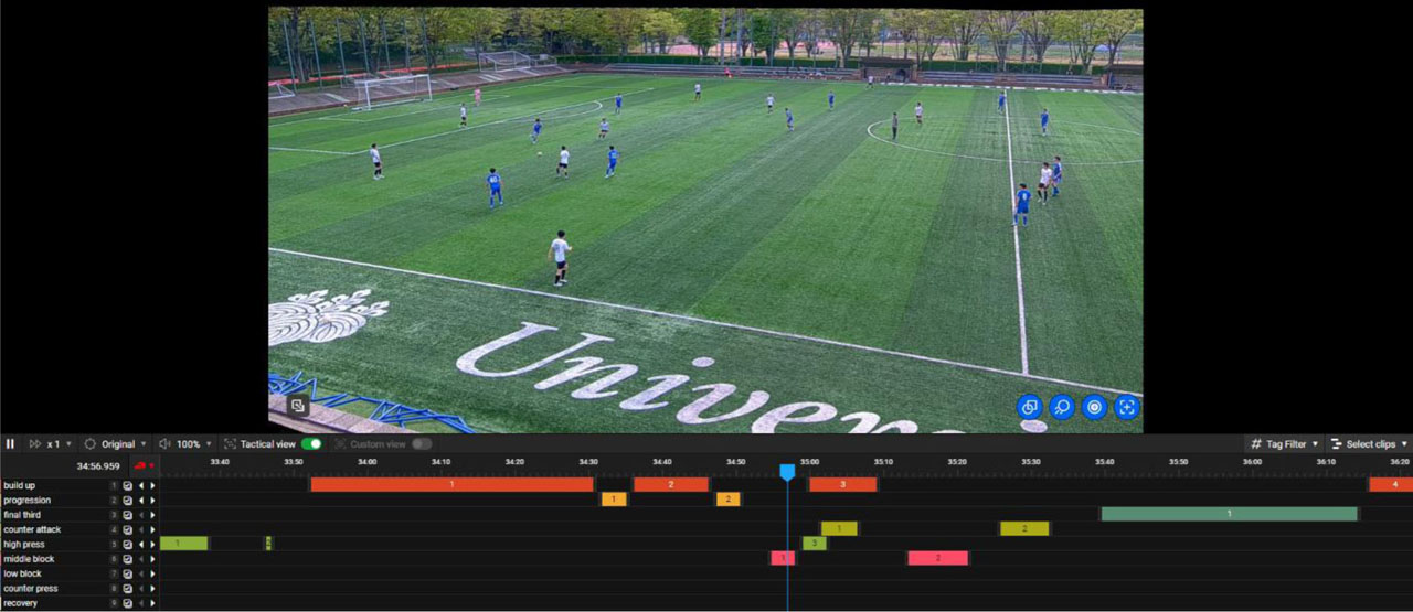
Figure A1:
Screenshot of the Bepro application used for play phase annotation by analysts.
Segment Assignment Optimization
To ensure a balanced distribution of play phases across the training, validation, and test sets, we formalize the segment assignment as an optimization problem based on tactical occurrence scores.
Phase Score Calculation
Let S = {s1, s2, … , sM} be the set of in-play segments. For each segment sj, we define a phase score vector vj = [vj,1, … , vj,9]T, where each element represents the combined score for a given phase across both teams. The score for a specific phase p in segment sj is calculated as the sum of its probabilities across all Wj frames within that segment:
where yu(p) ∈ {0.00, 0.25, 0.50, 0.75, 1.00} represents the annotated probability of phase p at frame u. The total cumulative score for phase p across the entire dataset is denoted as .Optimization Objective
We assign each segment to one of the groups G ∈ {train, valid, test} with target ratios rG ∈ {0.8, 0.1, 0.1}. The ideal score for phase p in group G is defined as Vp × rG. Let VG = ∑g∈G vg be the accumulated score vector for group G.
To minimize the discrepancy between the actual and ideal distributions, we greedily assign each segment sj to the group G that minimizes the following quadratic error function E:
Weighted Processing Order
To prevent statistical bias in rare phases, segments are processed in descending order of their total relative scarcity across all phases, calculated as . This priority ensures that segments containing infrequent phases, such as counter-attacks, are allocated to the training, validation, or test sets first, thereby maintaining a balanced representation of rare events across all subsets.
The resulting distribution of play phases across the training, validation, and test sets is presented in Table A2.
Table A2:
Evaluation of the segment assignment optimization across training, validation, and test sets. The scores for each play phase represent the sum of probabilities across all frames and both teams. Values in parentheses denote the ideal scores calculated as Vp × rG.
| Split | Total | Train (rG = 0.8) | Validation (rG = 0.1) | Test (rG = 0.1) |
|---|---|---|---|---|
| Number of Segments | 107 | 85 | 11 | 11 |
| Number of Sequences | 50553 | 40521 | 4874 | 5158 |
| Score of Build up | 22092.25 | 17761.25 (17673.80) | 1917.75 (2209.22) | 2413.25 (2209.22) |
| Score of Progression | 7435.00 | 6066.25 (5948.00) | 886.75 (743.50) | 482.00 (743.50) |
| Score of Final third | 7598.00 | 6007.75 (6078.40) | 830.25 (759.80) | 760.00 (759.80) |
| Score of Counter-attack | 4079.25 | 3035.25 (3263.40) | 516.75 (407.93) | 527.25 (407.93) |
| Score of High press | 6212.00 | 4911.00 (4969.60) | 715.25 (621.20) | 585.75 (621.20) |
| Score of Mid block | 13395.50 | 10530.75 (10716.40) | 1358.00 (1339.55) | 1506.75 (1339.55) |
| Score of Low block | 9931.75 | 8214.50 (7945.40) | 763.50 (993.18) | 953.75 (993.18) |
| Score of Counter-press | 4866.25 | 4098.75 (3893.00) | 413.75 (486.62) | 353.75 (486.62) |
| Score of Recovery | 4590.50 | 3496.25 (3672.40) | 621.00 (459.05) | 473.25 (459.05) |