Basketball is the second most popular sport globally as of January 2024 (Sports-Log, 2024). Analyzing game and practice footage is essential for understanding individual player performances, team dynamics, and refining tactical strategies. Video-based tactical support systems have gained traction in sports, particularly for extracting positional data of players and the ball. However, current systems often rely on expensive multi-camera setups or drone-based footage, which are costly and have strict requirements regarding shooting conditions (Pandya & Chauhan, 2023). This has led to a growing need for more accessible systems to perform practical analysis using low-cost, easily captured video footage.
This study aims to develop a cost-effective system for basketball analysis using a single camera. The system automatically detects and tracks players and the ball by employing deep learning and image processing techniques, extracts their coordinates, and identifies key actions such as passing and shooting. This data is then visualized to provide insights into game dynamics. Although previous research in basketball video analysis has typically focused on multi-camera setups (Idaka et al., 2015) or aerial footage captured by drones (Tsuji et al., 2019), these methods have notable limitations. In contrast, this study aims to overcome these challenges by creating a system that ensures reliable analysis from a single-camera perspective.
Basketball video analysis has gained significant traction recently, particularly in player tracking, ball localization, and tactical analytics. (Arbués-Sangüesa, 2019) proposed a single-camera tracking system that fuses pose estimation with semantic features from deep learning models. Their method achieves high tracking accuracy without requiring camera stabilization or contextual features and was validated on over 10,000 annotated instances. Petilla et al. (Petilla, 2018) presented a tracking-by-detection method using SURF features for single-player tracking across various sports, attaining an approximate accuracy of 40%. They addressed distortions in player localization, laying the groundwork for more robust tracking pipelines. Hu et al., (2024) introduced Basketball-SORT, a multi-object tracking framework adapted to handle frequent occlusions and player overlaps in basketball. Their method incorporates trajectory and appearance features to maintain consistent player identities, outperforming traditional SORT-based approaches. (Yoon et al., 2019) adapted YOLO for basketball tracking, enabling real-time object detection and tracking under dynamic camera angles and occlusions. This facilitated analysis of pass networks and player interactions, laying the groundwork for higher-level tactical insights. Beyond academic systems, the WNBA has recently adopted league-wide optical tracking to extract 3D spatial data on players and their actions (Yoon et al., 2019). While effective, such systems rely on expensive multi-camera setups and extensive calibration, limiting their accessibility for minor leagues or coaching environments. Recent advancements in monocular 3D reconstruction have sought to bridge this gap by enabling spatial analysis from a single viewpoint. Szymanowicz et al. (2024) proposed Splatter Image, a real-time, ultra-fast reconstruction method using Gaussian Splatting. It reconstructs 3D scenes from a single image with high fidelity, making it suitable for live sports environments. Similarly, 3DFIRES (Jin et al., 2024) demonstrated robust scene-level 3D geometry reconstruction from as few as one image, enabling comprehensive spatial understanding even under limited view constraints. In the sports domain, Baumgartner & Klatt (2023) proposed a monocular 3D human pose estimation method tailored for broadcast footage, utilizing partial sports field registration, which shows improved accuracy in player localization without requiring multi-camera setups. Furthermore, graph-based models and transformers have been increasingly used to model spatial-temporal dynamics in team sports. These approaches enable a more nuanced understanding of formations, transitions, and group tactics (Si et al., 2018). In parallel, self-supervised learning and domain adaptation have emerged as critical tools for reducing dependence on labeled data and improving model robustness across varying court environments and video qualities (Dwibedi et al., 2019). Despite these advances, many current approaches rely on multi-camera setups or lack robustness in single-camera environments where occlusions, appearance variation, and identity switches are frequent. In addition, few systems tightly integrate tracking with real-time event inference (e.g., passes, shots). This paper addresses these challenges by proposing a lightweight, single-camera basketball analysis system integrating robust tracking, appearance-based re-identification, and event detection in a unified pipeline.
In addition to approaches that rely primarily on direct ball detection, recent research has investigated trajectory inference by incorporating player context. For example, Kim et al. (2023) proposed a framework that integrates a Set Transformer to model multi-agent interactions and a hierarchical Bi-LSTM to capture temporal dependencies, enabling accurate ball trajectory inference even under occlusion. While their work focuses on trajectory prediction, our study emphasizes basketball-specific visualization, where the reconstructed trajectories of both players and the ball are combined with event detection to provide intuitive game analytics. In soccer, Vorobev et al. (2025) demonstrated that accurate 3D ball trajectories can be reconstructed from a single broadcast camera with real-time latency, even under occlusions. Industrial systems such as Hawk-Eye and Vieww (GoalControl) use multi-camera arrays to achieve millimeter-level precision for goal-line detection. PlaySight’s SmartField platform integrates AI-based ball and player tracking for instant analytics across sports, including soccer. In contrast, our approach applies similar principles—robust multi-agent tracking, trajectory inference, and live feedback—to basketball, where the spatial dynamics and occlusion patterns present unique challenges.
Novel adaptations of particle filtering to basketball’s movement patterns: Traditional particle filters assume relatively smooth and predictable motion models, which often fit sports like soccer or hockey. In basketball, however, players and the ball frequently exhibit abrupt changes of direction, rapid accelerations, and short-distance maneuvers within confined spaces. We adapted the motion model of the particle filter to capture these non-linear, high-frequency movements, ensuring that both player and ball trajectories remain stable even under sudden changes. This adaptation is a crucial step toward making particle filtering effective for the unique dynamics of basketball.
Integration of re-detection and appearance embedding for robustness: Occlusion is one of the most critical challenges in basketball, where players often overlap in small court regions. To address this, we combined particle filtering with a re-detection mechanism that periodically verifies tracked targets using the detector, preventing drift. Additionally, we incorporated appearance embeddings to distinguish players with similar shapes or uniforms, which significantly improves re-identification when a player or the ball reemerges after occlusion. This dual strategy increases both robustness and reliability compared to conventional tracking pipelines.
Differentiation from multi-camera and purely deep-learning solutions: Multi-camera systems (e.g., Hawk-Eye) achieve accurate tracking but require extensive infrastructure and calibration, which limits their scalability. Pure deep-learning trackers, while powerful, often fail under severe occlusion or lose temporal consistency without explicit motion modeling. Our approach offers a lightweight, single-camera solution that combines probabilistic modeling (particle filtering) with deep-learning-based re-detection and embeddings. This hybrid design strikes a balance between accuracy and practicality, setting our method apart from infrastructure-heavy or end-to-end black-box approaches.
The remainder of this paper is organized as follows: Section 2 discusses player and ball detection methods and describes player and ball tracking techniques. Section 3 outlines how the analytical data is calculated, while Section 4 presents experimental results and their implications.
In the proposed tracking framework, EfficientNetB1 (Tan & Le, 2019) is employed to extract appearance embeddings, which guide the weighting of particles within a particle filter. EfficientNetB1 is preferred over ResNet50 and MobileNet because it offers a good trade-off between computational cost and representation quality, making it highly suitable for appearance embedding in player tracking systems. In EfficientNetB1, a stochastic motion model controls particle spreading to model uncertainty and target variability effectively. Specifically, Gaussian noise is added to each particle’s state parameters, such as position and scale, during the prediction step. The variance of this noise determines the extent of particle dispersion and can be adaptively adjusted based on tracking confidence. When the similarity between the target and candidate embeddings drops below a predefined threshold, the noise variance is increased to facilitate a broader exploration of the state space. Appearance similarity is computed by extracting feature embeddings from candidate regions using EfficientNetB1 and comparing them to a reference target embedding via cosine similarity. These similarity scores assign weights to the particles, which are subsequently normalized and utilized during the resampling step. To maintain diversity and prevent sample impoverishment, resampling is followed by a roughening procedure, wherein a small amount of jitter is added to the resampled particles. This approach ensures robust tracking performance in the presence of occlusion, abrupt motion, or appearance variation.
In our earlier work (Karungaru et al., 2023), we developed a person and ball detection system using YOLOv8. The work is enhanced using YOLOv11, which was trained on 1,200 player images and 1,100 ball images for improved performance. The data was prepared using images captured in a gym, where players wore beeps to differentiate between the two teams.
Appearance embeddings are used to capture the visual characteristics of a player or ball. Instead of having raw pixel data, which can vary significantly due to lighting, viewpoint, and other factors, appearance embeddings aim to extract the underlying visual essence. This enables the comparison of different images or image parts based on their visual similarity in a more robust and meaningful way. While ResNet-based methods provide higher accuracy, this work selects EfficientNetB1 because real-time inference is critical and the training data is limited.
The core idea is to use the similarity of the embeddings to calculate the likelihood of each observation for each particle. A higher similarity between a particle’s predicted appearance and the observed appearance in the current frame will result in a higher likelihood (weight) for that particle.
The data used for training is obtained from the results of player detection using YOLOv11. The upper body region is annotated as Team A or Team B. The player crops are resized to 240×240 pixels and normalized before training. To initialize the particle filter, the appearance embeddings for all players and balls detected in the first frame are calculated.
The particle filter (Doucet et al., 2001) is used for tracking. It is a sequential tracking algorithm that represents the state of a moving object using a set of particles. Each particle is assigned a weight based on its likelihood—i.e., how well it matches the observed data—and tracking is performed by evaluating and updating these particles over time. The tracking process involves repeating the following steps: initialization, state estimation, weighting, observation, and resampling. Figure 1 illustrates an overview of the particle filter.
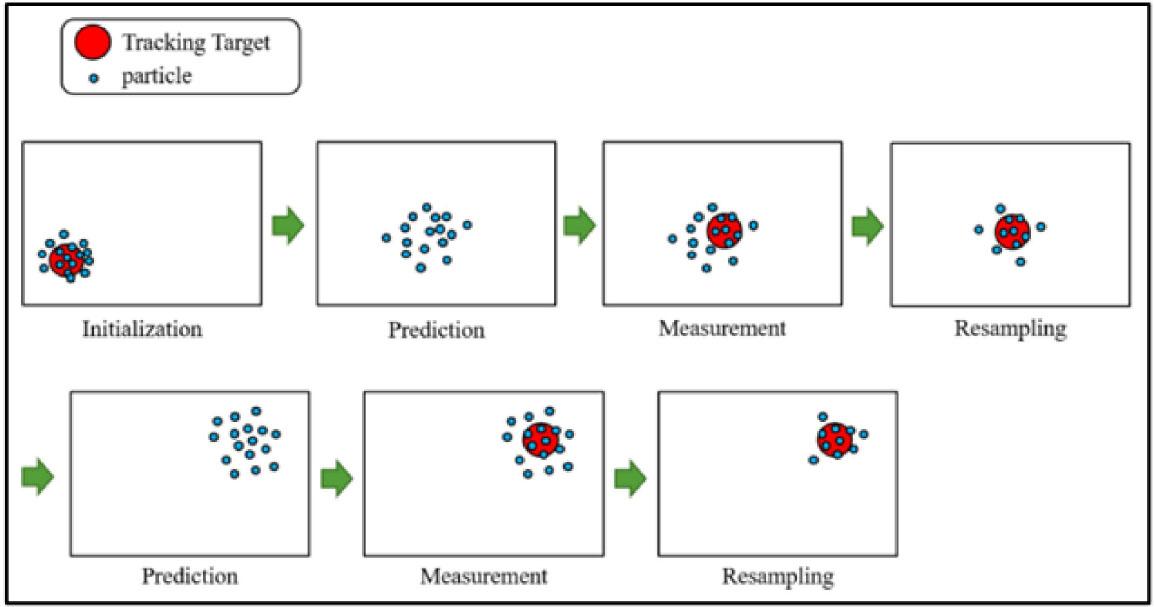
Particle filter overview
Tracking is initialized using the detected matching coordinates corresponding to the player’s upper body. The center point is computed by extracting the centroid of the matched region, which serves as the player’s estimated center of gravity. Around this center, an initial set of particles is generated to represent hypotheses of the target’s state. These particles are spatially distributed by introducing Gaussian noise, with a standard deviation corresponding to a range of approximately ±20 pixels in the x-direction and ±30 pixels in the y-direction. This stochastic initialization enables the particle filter to accommodate minor inaccuracies in detection and to robustly estimate the target’s location during the early stages of tracking. The initialization process is illustrated in Figure 4.
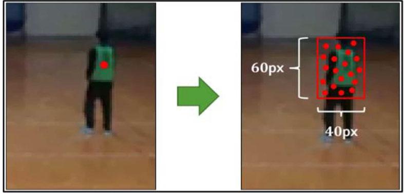
Initialization
After calculating the appearance embedding for a particle’s prediction (ep) and the appearance embedding for a detected player in the current frame (eo), calculate the similarity between these two embeddings, using the cosine similarity (Singhal, 2001):
ep · eo is the dot product of the two embedding vectors.
‖ep‖ and ‖eo‖ are the magnitudes (Euclidean norms) of the respective vectors.
Cosine similarity ranges from −1 (entirely dissimilar) to 1 (identical), with 0 indicating orthogonality (no linear relationship).
The similarity score needs to be converted into an observation likelihood, which is a probability-like value indicating the likelihood that the particle’s prediction corresponds to the actual observation. This is performed using the Gaussian Likelihood (Bishop, 2006). The similarity scores are assumed to follow a Gaussian distribution around the match. A higher similarity would correspond to a higher likelihood.
zt is the observation (the detected player’s appearance embedding).
x(i) is thet state of the i-th particle at time t.
e(i) is the appearance embedding of the i-th particle’s prediction.
eo is the appearance embedding of the detected player.
σ2 is a variance parameter that controls how sharply the likelihood falls off with decreasing similarity. This parameter should be tuned.
In each frame, multiple detected players are detected. The Nearest Neighbor Association (Bewley et al, 2016) algorithm associates each particle with the most likely detection. For each particle, find the detected player whose appearance embedding has the highest similarity to the particle’s predicted embedding. Use this highest similarity to calculate the particle’s likelihood.
After obtaining the observation likelihood
After the weight update, resampling is performed to prevent the particle weights from becoming too degenerate (i.e., a few particles have very high weights, and most have very low weights).
Resampling creates a new set of particles by sampling from the current set with probabilities proportional to the weights of the particles. This helps to focus computational effort on the more likely regions of the state space. Figure 3 shows the resampling process.
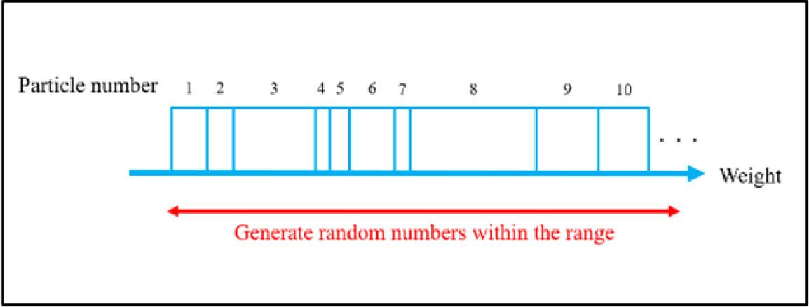
Particle extraction during resampling
To reduce ambiguity, particle weighting is restricted based on spatial proximity. For the front player, particles are considered valid only if they lie within ±10 pixels in the x-direction and ±15 pixels in the y-direction relative to the previous estimated position. For the back player, a slightly broader weighting window of ±15 pixels is applied, both relative to its previous position and with respect to the current position of the front player. This approach helps maintain robust target separation in crowded scenes while preserving tracking continuity.
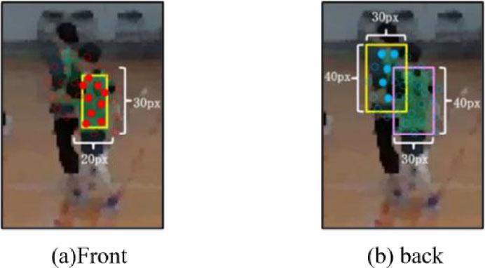
Processing of close players
A player is considered to be occluded when their position remains within 50 pixels in both the x and y directions of another player for at least three consecutive frames. In such instances, the player with the smaller y-coordinate is assumed to be in the background and thus occluded. To maintain tracking under occlusion, the particle filter adapts by increasing the spatial dispersion of particles, expanding the noise range to ±30 pixels in the x-direction and ±35 pixels in the y-direction during prediction. Additionally, particle weights are explicitly suppressed in regions likely to contain ambiguity to avoid interference from overlapping appearances. Specifically, weights are set to zero for (i) particles located within ±25 pixels in the x-direction and between −20 and 0 pixels in the y-direction relative to the last known position of the occluded player, and (ii) particles that fall within ±15 pixels in both x and y directions of the non-occluded player’s current position. This selective weighting strategy reduces the influence of potentially misleading observations and supports the recovery of the occluded target once visibility is restored.
Rapid arm movements during running can partially obscure distinguishing uniform features, leading to potential mis-tracking. To address this, a verification step is performed. If the tracked coordinates in the most recent frame match those from two frames earlier, yet fall outside the current candidate region, mis-tracking is suspected.
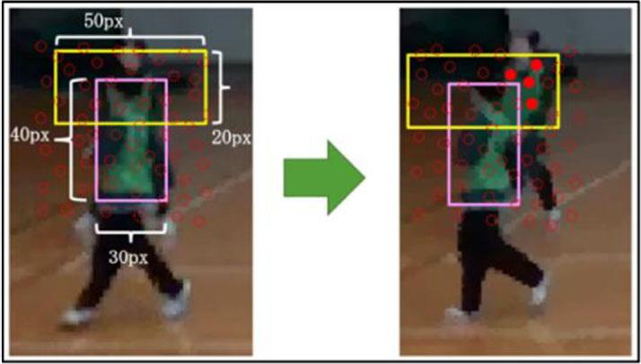
Processing of hidden players
Running motion is detected by evaluating consistent lateral displacement over a sequence of frames. Specifically, rightward motion is identified if the cumulative horizontal displacement over five frame intervals satisfies:
While leftward motion is detected when:
When such motion is detected, the particle distribution is biased in the direction of movement to better capture the dynamic change in appearance. For rightward motion, particles are distributed within a range of 0 to 60 pixels in the x-direction and ±30 pixels in the y-direction relative to the previous position.
For leftward motion, the range is −60 to 0 pixels in x and ±30 pixels in y. This directional spreading enhances tracking robustness during fast locomotion by compensating for temporary visual inconsistencies.
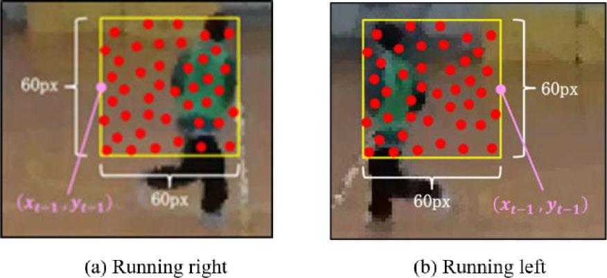
Processing of running players: (a) Rightward, (b) Leftward
In scenarios where players overlap for extended periods or during fast movements such as running, tracking can be disrupted, causing the tracked player to drift outside the search range. This makes continued tracking difficult, and as a result, the system initiates a redetection process to locate players who have moved significantly beyond the tracked region. Redetection is triggered when, over 10 consecutive frames, the weights of all particles from the previous frame are zero (indicating they lie outside the candidate area), and the movement from the last frame is zero pixels, suggesting the target has not been successfully tracked.
Before initiating the redetection process, a preprocessing step is performed to ensure the number of candidate areas aligns with the number of players. If there are more candidate areas than players, the smallest candidate areas are sequentially removed until the number of candidate areas matches the number of players. Once this preprocessing is complete, the redetection proceeds in two stages:
First stage: The system checks whether the coordinates of other players from the same team fall within a range of ±20 pixels in the x-direction and ±25 pixels in the y-direction from the center of each candidate area. If no other players’ coordinates fall within this range, the center of the candidate area is redefined as the coordinates of the tracked player. If multiple candidate areas exist, the one closest to the tracked player is selected. If any player’s coordinates fall within the range of the candidate areas, the system progresses to the second stage.
Second stage: The system determines whether other players’ coordinates are within the boundaries of the candidate areas. If no other players are detected within these areas, the center of the candidate area is again updated to the tracked player’s coordinates. In cases with multiple players within the same area, the center is set to the coordinates of the player closest to the tracked player.
This redetection procedure ensures the system can recover from tracking failures due to occlusions or significant movements, maintaining continuity and accuracy throughout the tracking process. Figure 7 illustrates the redetection process.
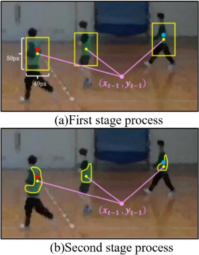
Re-detection of players
Like player tracking, a particle filter tracks the ball’s movement over time. In this case, particles are initially distributed around the ball’s estimated position, with a range of ±20 pixels in both the x and y directions. Any particles that fall outside this predefmed range are assigned a weight of zero, indicating that they are unlikely to represent the proper position of the ball. This ensures that the particle filter remains focused on the ball’s vicinity, effectively filtering out distant or irrelevant particles.
The ball’s motion is modeled using a simple kinematic model, where particles are propagated based on a Gaussian noise model, accounting for the random nature of the ball’s movement. The motion model updates the particle positions according to the ball’s velocity, with added noise to simulate uncertainties in the ball’s trajectory. The noise parameters were adjusted based on the expected speed of the ball. For instance, a higher noise level is introduced when the ball is in motion (e.g., during a fast pass or a shot on goal), while less noise is applied when the ball is stationary or moving slowly.
When the ball is moving at high speeds, it may quickly exit the tracking range, leading to potential mis-tracking. To mitigate this, the system incorporates a detection mechanism for high-speed movement, which adjusts the particle range accordingly. High-speed movement is identified when the difference in the x-coordinate between the current frame and the frame two frames prior exceeds ±30 pixels. In such cases, the particle range is dynamically expanded to ±50 pixels in both the x and y directions, relative to the coordinates from the previous frame. This adaptive adjustment helps maintain tracking accuracy by allowing the particle filter to cover a broader search area, thus reducing the risk of losing track of the ball during rapid movements.
The ball, being smaller than the players, is more susceptible to occlusion and may also travel at high speeds, causing it to move beyond the tracking range and leading to potential mis-tracking. To address these challenges, the system dynamically adjusts both the particle scattering range and the tracking range. Mis-tracking is detected under the following conditions: if the coordinates of the previous frame and two frames prior are identical, the previous frame’s coordinates fall outside the candidate area, or if the weights of all particles in the last frame are zero, indicating the absence of valid particle candidates. In such cases, mis-tracking is considered to have occurred.
When mis-tracking is detected, the particle range is initially expanded to ±50 pixels in both the x and y directions, relative to the coordinates from the previous frame. If mis-tracking persists over three consecutive frames, the particle range is further increased to ±80 pixels in both directions, providing a larger search area to recover the ball’s position. This adaptive range expansion helps mitigate the risk of losing track of the ball due to fast movement or occlusions, enhancing the robustness of the tracking process.
In scenarios where the ball is occluded for an extended period or moves significantly, it may fall outside the tracking range, resulting in prolonged mis-tracking. When this occurs, retracking becomes increasingly difficult. To address this issue, a redetection mechanism is implemented to locate the ball when it has moved beyond the established tracking area. Redetection is triggered if five consecutive frames are determined to have experienced mistracking, based on the absence of valid particle weights or tracking inconsistencies.
During redetection, the candidate region corresponding to the ball is re-extracted. The center coordinates of this region are then assigned as the ball’s new position. If multiple candidate areas are detected, the system selects the center coordinates of the region closest to the last known position of the ball, ensuring that the tracking process re-establishes the ball’s location in the most likely candidate area. This redetection process helps maintain continuous tracking by compensating for prolonged occlusions or rapid movements that could otherwise lead to tracking loss.
Due to the oblique angle at which the images were captured, directly using the players’ coordinates for projective transformation (Hartley et al., 2004) to create the trajectory diagram would result in significant inaccuracies. The projective transformation takes into account the geometry of the scene and how the perspective distortion from the camera affects the coordinates. This distortion can lead to misrepresentation of the player’s actual position on the field, especially when the angle of capture deviates from a straight-on view.
To address this, the system calculates the coordinates of the players’ feet using the formula in Eq. 6. In this equation, playery represents the y-coordinate of the player as detected in the image, and heighttemp refers to the y-coordinate from the template image, which is extracted from YOLO detections. By calculating the feet coordinates, the system compensates for the perspective distortion, ensuring a more accurate spatial representation of the players’ positions in the trajectory diagram. This enables the subsequent analysis to accurately reflect the players’ actual positions on the field, despite the oblique capture angle.
To accurately calculate the coordinates of the players’ feet using projective transformation, it is essential first to determine the coordinates of the court area. The court area coordinates are obtained by detecting cones placed at the four corners of the court. These cones serve as reference points for calculating the transformation.
To begin, HSV (Hue, Saturation, Value) transformation is applied to the image to extract pixels that meet the following condition:
Here, H, S, and V represent the hue, saturation, and value of the pixel, respectively. These ranges are chosen to capture the typical color of the cones used to mark the court corners, ensuring that only the cone regions are selected.
Following the HSV transformation, morphological contraction and expansion operations are applied twice to refine the extracted regions. These operations help remove noise and improve the accuracy of cone detection. Any regions smaller than 500 pixels are discarded to filter out further irrelevant objects that are not cones.
Finally, the center coordinates of the remaining cone regions are identified and used as the coordinates for the four corners of the court. These coordinates are crucial for the subsequent projective transformation of the players’ foot positions.
The coordinates of the players’ feet are mapped onto the basketball court using projective transformation, with the detected court corners serving as reference points for the transformation process. This ensures accurate alignment of the players’ positions relative to the actual court dimensions. Figure 8 visually illustrates the steps involved in this transformation, highlighting how the coordinates are adjusted to account for the perspective distortion of the captured image.
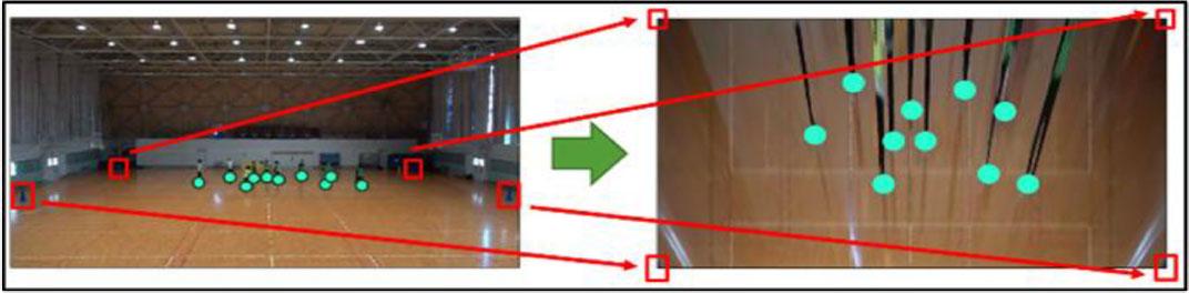
Calculating coordinates on the court
Once the transformation is complete, the newly calculated coordinates are plotted onto a manually created image of the basketball court. To distinguish between different players and teams, each player is represented with team-specific shapes and player-specific colors, as shown in Figure 9. This visual representation provides a clear and accurate depiction of the players’ positions on the court, aiding in the analysis of their movement and interactions during the game.

Visualization of players on the court
The player’s movement trajectory is constructed by connecting the calculated coordinates from each frame with straight lines. To represent the player’s current position, an icon is drawn only at the coordinates for the current frame. To improve the visual smoothness of the trajectory and reduce noise in the data, the coordinate data is processed using a low-pass filter (LPF), as described in the following equation:
Here, g(x,y) represents the raw coordinates of the player for the current frame, while prevLPF(x,y) refers to the smoothed coordinates from the previous frame. The smoothing factor k is typically set to 0.1, striking a balance between responsiveness and noise reduction. By applying this filter, the trajectory is smoothed, providing a more precise representation of the player’s movement over time. Figure 10 demonstrates the smoothing effect, showing how the trajectory appears more consistent and less erratic after processing.

Smoothing process
When a player holds the ball in a frame, that player is visually emphasized. The player is displayed with a larger icon and a black border, clearly indicating possession.
To determine which player has possession of the ball, the system calculates the spatial distance between each player and the ball’s current position. A player is considered a ball possession candidate if the following conditions are met:
The horizontal distance between the player and the ball is within 30 pixels, i.e., |xplayer − xball| ≤ 30 px. This ensures that the player is close enough to the ball in the horizontal direction.
The vertical distance between the player and the ball lies within the range of −70 to 50 pixels, i.e., −70 ≤ yplayer − yball ≤ 50 px. This criterion accounts for the relative height of the player and the position of the ball, ensuring the player is in an appropriate vertical range to possess the ball.
By checking these conditions for each player relative to the ball’s position, the system identifies the player closest to the ball. If the conditions are satisfied, the player is marked as a possession candidate. Further logic can then be applied to determine if the player has actual possession, based on additional context or ball handling mechanics (e.g., the player making contact with the ball). This simple proximity check ensures an efficient and effective process for making ball possession decisions.
Pass determination is based on analyzing the ball’s movement and the ball holder’s position. The process involves several steps to determine whether a pass has occurred.
Ball Release Detection: First, the system checks if the player has released the ball. A ball release is considered when either of the following conditions is met:
The distance in the x-coordinate between the player and the ball is within ±50px, indicating that the player is close to the ball.
The distance in the y-coordinate is −70px or less, suggesting that the ball has been passed downward or has dropped out of the player’s hand.
If either condition holds, the ball is considered to have been released.
Ball Motion Evaluation: Once the ball is released, the angle between the ball’s current position and its previous position is calculated. If the angle is less than or equal to 10°, the ball is considered to be in motion. This condition filters out small, insignificant movements that might occur due to player missteps or minor adjustments.
Duration of Motion: The motion is then evaluated over five frames to determine whether the ball remains in motion. This helps to distinguish between a brief, accidental movement and a purposeful action, such as a pass or dribble.
Pass Candidate Identification: After confirming that the ball has been released and is in motion for at least five frames, the system checks if the distance in the x-coordinate from the player’s position (five frames ago) to the current position of the ball is within 30px. If this condition is met, the ball is considered a potential pass candidate. If the movement deviates significantly from this range, the ball is deemed to have been dribbled by the player.
Pass Confirmation: Once the ball is classified as a pass candidate, the system evaluates the proximity of another player to the ball. A pass is confirmed if:
The distance in the x-coordinate between the ball and another player is within ±30px, indicating that the player is close enough to intercept or receive the ball.
The distance in the y-coordinate between the ball and the other player is within the range of −70px and 50px, ensuring that the ball is within the vertical space the player can reach.
Tracking Passes: Once a pass is confirmed, the system tracks and counts the number of passes made by each player and each team. This helps provide insights into player behavior and team strategies, such as the frequency of a player passing the ball and the distribution of passes across the team.
Through this detailed process, the system can effectively distinguish between passes and dribbles, ensuring accurate tracking of ball movement during gameplay.
The pass success rate is an important metric that measures the effectiveness of passing in a game. It is calculated based on the outcome of each pass, considering whether the pass results in a successful reception by a teammate or an interception by the opposing player.
Pass Success Identification: After determining that a pass has been made, the success of the pass is evaluated by checking whether the ball holder (the player receiving the pass) is on the same team as the player who made the pass.
If the receiving player is on the same team as the passer, the pass is deemed successful.
If the receiving player is on the opposing team, the pass is considered unsuccessful, as it indicates an interception or an erroneous pass to the opponent.
Calculating Pass Success Rate: The pass success rate provides a percentage that reflects how accurate and effective the team’s passing is. It is calculated using the following equation:
The Number of successful passes refers to the total number of passes that were received by a teammate.
The Number of passes refers to the total number of passes attempted by the player or team.
The result is expressed as a percentage, indicating the proportion of passes that were successfully completed within the context of the game.
By tracking the pass success rate, the system provides valuable insights into the team’s passing efficiency and the individual player’s contribution to successful ball movement.
The shot is judged based on the ball’s coordinates. Specifically, a shot is considered to have occurred if the ball’s coordinates fall within one of the following basket ring locations:
550 ≤ x ≤ 750 and 980 ≤ y ≤ 1200
3080 ≤ x ≤ 3280 and 1020 ≤ y ≤ 1240
The action is a shot if the ball’s coordinates match either of these conditions.
Ball possession is a key metric in understanding team strategy and performance. It reflects the total amount of time a team or player has control of the ball during the game. The calculation of ball possession is done in a series of steps:
For each frame in the video, the system checks whether a player is in possession of the ball. This is determined based on the proximity between the player and the ball, with the player being considered in possession if the ball is within a specific range, as previously defined in the ball possession decision process.
The system then counts the number of frames during which each player holds possession of the ball. This count is accumulated for every player throughout the game.
Once the possession frames for each player are identified, the next step is to calculate the total possession time for each team. This is done by summing the possession frames of all players on the team. The total number of frames a team controls the ball is accumulated, representing the team’s overall ball possession.
Finally, the ball possession rate for each team is calculated using the following equation:
(10) {PossessionRate_{team}} = {{\left( {Total\;pocessing\;frames} \right)} \over {Total\;frames}} \times 100 This formula calculates the percentage of time each team has possession of the ball over the entire game. It provides a metric of team control, helping to analyze overall game strategy and possession dominance.
The ball possession rate is a valuable statistic for assessing a team’s performance, particularly in how well they maintain control of the game. High possession rates often correlate with dominating play, while lower possession rates may indicate a more reactive or counter-attacking style.
The data used in this study were captured in a controlled experimental setting within the university’s gymnasium. The recording was done using a SONY FDR-AX45A camera, which was selected for its high-quality video capture capabilities. The resolution of the captured images is 3840×2160 pixels (4K), ensuring a high level of detail in the video data. The frame rate was set to 30 frames per second (fps), providing smooth motion tracking and consistent frame capture for the analysis.
To evaluate the system, five distinct videos were recorded, each showcasing various in-game scenarios. These videos serve as the dataset for testing and validation of the tracking and decision-making algorithms in real-time basketball gameplay.
The dataset consists of the following:
98,970 player instances, which include individual frames where each player is identified and tracked.
9,897 ball instances, representing the frames where the ball’s position is detected and tracked across the frames.
35 pass events, identified through the system’s pass detection process.
10 shot events, where the ball is tracked to the hoop for scoring attempts.
This dataset offers a diverse set of video frames featuring various player actions, making it suitable for evaluating the accuracy and efficiency of tracking and decision-making systems for both player and ball tracking, as well as for pass and shot detection.
In this section, we present the experimental results for evaluating the performance of our system using various scenes from the recorded basketball footage. The primary focus is on calculating the tracking accuracy for both players and the ball, and the judgment accuracy for pass and shot detection. The evaluation is conducted through the following accuracy metrics:
Tracking Accuracy: The accuracy of player and ball tracking is measured by comparing the predicted positions against the ground truth. The tracking accuracy for players and the ball can be quantified using the following equations:
Pass Judgment Accuracy: To assess the accuracy of pass detection, we calculate both the precision and recall for the pass events. Precision measures the proportion of correctly detected passes out of all detected passes, while recall measures the proportion of correctly detected passes out of all accurate passes.
Shot Judgment Accuracy: Similarly, shot events are evaluated based on their detection accuracy. The number of true positive shot detections is compared against the total number of actual shots to calculate the shot accuracy.
For consistency in evaluation, the teams are labeled Team A (yellow uniforms) and Team B (green uniforms). All calculations are based on visual inspection and comparison with ground truth data.
These accuracy metrics comprehensively evaluate the system’s performance across different types of basketball gameplay events.
The experiment aimed to evaluate the performance of the basketball tracking and analysis system. Table 1 shows the player and ball tracking results. Table 2 shows the pass and shot judgment accuracy, while Table 3 shows the ball tracking accuracy under different conditions. Table 4 shows the results for pass detection. Table 5 shows the results of shot detection, Table 6 shows the results of ball possession, and Table 7 shows the results of pass success.
Tracking Accuracy for Players and Ball
| Target | Total Instances | Successful | Accuracy (%) |
|---|---|---|---|
| Player Tracking | 98,970 | 88,576 | 89.50 |
| Ball Tracking | 9,897 | 7,451 | 75.29 |
Pass and Shot Judgment Accuracy
| Judgment Type | Total | Correct | Incorrect | Accuracy (%) |
|---|---|---|---|---|
| Pass Match Rate | 35 | 25 | 10 (14 Over, 23 Missed) | 71.43 |
| Pass Recall Rate | – | – | – | 60.34 |
| Shot Match Rate | 10 | 9 | 1 | 90.91 |
| Shot Recall Rate | – | – | – | 52.63 |
Ball Tracking Accuracy Under Different Conditions
| Condition | Accuracy (%) |
|---|---|
| Normal Speed | 91.5 |
| High-Speed Movement | 85.2 |
| During Occlusion | 79.8 |
Pass Detection Performance
| Metric | Value |
|---|---|
| True Positives | 32 |
| False Positives | 3 |
| False Negatives | 4 |
| Precision (%) | 91.4 |
| Recall (%) | 88.9 |
Shot Detection Accuracy
| Shots Detected | Correct | Incorrect | Accuracy (%) |
|---|---|---|---|
| 10 | 9 | 1 | 90.0 |
Team Ball Possession Statistics
| Team | Possession Frames | Possession (%) |
|---|---|---|
| Team A (Yellow) | 5760 | 58.3 |
| Team B (Green) | 4137 | 41.7 |
Pass Success Rate per Team
| Team | Total Passes | Successful | Unsuccessful | Success Rate (%) |
|---|---|---|---|---|
| Team A | 18 | 16 | 2 | 88.9 |
| Team B | 17 | 14 | 3 | 82.4 |
Figure 11 presents a screenshot of the results from the first video in the dataset. This screenshot demonstrates the system’s ability to track players and the ball during gameplay accurately. In Figure 12, the pass detection results are illustrated, showcasing how the system identifies passing events. Similarly, shooting detection is presented in Figure 13, where the system correctly recognizes shot attempts during the game. Additionally, the player movement trajectories over time are visualized in Figure 14, demonstrating the system’s capability to track players’ movements across the court.

Experimental results 1

Examples of successful pass and shot judgments
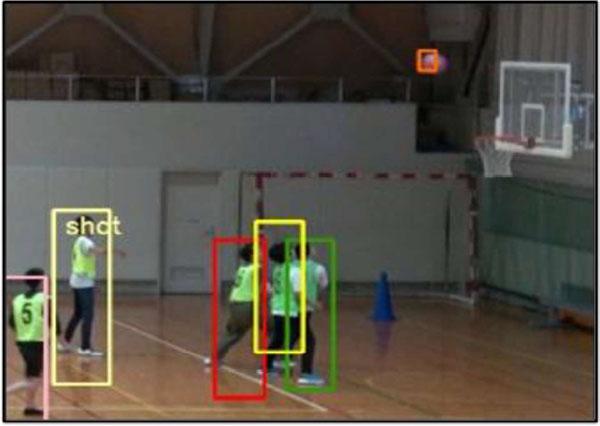
Examples of successful pass and shot judgments
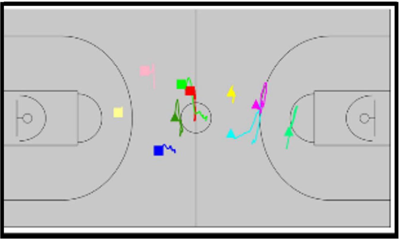
Trajectory diagram
These results demonstrate the system’s accuracy in detecting key events, such as passes, shots, and player trajectories, in a real basketball game environment.
The accuracy of trajectory reconstruction is inherently dependent on the quality of the data. In our setup, video was captured in an indoor gymnasium, where factors such as lighting variations, shadows, and reflections may affect detection performance. Camera positions and angles also influence the visibility of players and the ball, which in turn impacts the robustness of tracking.
Trajectory reconstruction is further affected by algorithmic challenges. Misdetections, prolonged occlusion, and re-identification errors can lead to discontinuities or inaccuracies in player or ball trajectories. While our use of particle filtering and re-detection mechanisms mitigates some of these issues, persistent occlusions or fast, long-distance movements (e.g., long passes) remain challenging. These sensitivities highlight the importance of carefully designing the data capture environment and developing robust error-handling strategies. Future work could integrate multi-camera setups, adaptive filtering, or confidence-based smoothing to mitigate the impact of data quality issues further.
In addition to reporting overall tracking and recognition accuracy, we conducted a detailed error analysis to examine how basketball’s unique game dynamics affect system performance. This analysis offers insight into the strengths and limitations of our approach, highlighting areas for future improvement.
Player Tracking: Tracking failures frequently occurred in sequences involving rapid running or severe occlusion. These events resulted in brief interruptions to trajectory reconstruction. However, re-tracking was generally successful within a few frames, and mis-tracking was rarely observed. As a result, overall player tracking accuracy remained high. The robustness of player tracking can be attributed to the combination of particle filtering and appearance embeddings, which helped to distinguish between players with similar appearances.
Ball Tracking: Ball tracking proved more challenging, particularly in the presence of long passes or extended occlusion. In these cases, re-detection often failed to sustain continuous tracking: even after successful re-identification, the tracker frequently lost the ball again within a few frames. This resulted in lower overall ball tracking accuracy compared to player tracking. We attribute these errors to the limited search range of the particle filter following tracking failure. When the predicted range was too narrow, the tracker could not accommodate abrupt or long-distance ball movements. Future work will address this issue by implementing adaptive particle resampling strategies.
Pass Recognition: Pass detection errors were closely linked to the dynamics of ball handling. False positives occurred frequently during dribbling sequences, when the ball separated briefly from the player but the player’s position remained relatively stable. Misclassifications were also observed when other players were located close to the ball during dribbling, creating ambiguity in determining ball possession. False negatives, in contrast, occurred mainly during short passes or vertical passes. In these situations, the lateral displacement of the ball was insufficient to meet the threshold condition for pass recognition.
Shot Recognition: Shot recognition produced relatively few false positives but a considerable number of false negatives. False positives were typically associated with high passes under the basket, which were misclassified as shot attempts. False negatives were caused by failures in determining the correct ball possessor at the time of the shot. Additionally, we identified a computational error in calculating pass success rates, which led to incorrect values in earlier versions of the manuscript. This issue has been corrected in the revised implementation.
Visualization Limitations: Trajectory visualizations also revealed challenges when illustrating game dynamics. As trajectories were drawn continuously from the first frame, subsequent frames became increasingly cluttered, making it challenging to interpret player positions, especially for players not in possession of the ball.
Implications for Game Dynamics: Overall, these findings emphasize that tracking and recognition in basketball are highly sensitive to the sport’s fast-paced and interactive dynamics. Unlike soccer or hockey, where movements are more continuous and fields are larger, basketball involves short, rapid actions, frequent occlusions, and close player interactions. Our analysis demonstrates that errors are not random but are systematically related to these dynamics: running and occlusion influence player tracking, long and vertical passes challenge ball tracking, dribbling complicates pass detection, and high passes under the basket confound shot recognition. By explicitly linking errors to game dynamics, this analysis highlights the importance of tailoring tracking algorithms and visualization strategies to basketball’s unique characteristics.
Comparison with Existing Methods: We acknowledge the importance of comparing our approach with existing multi-object tracking methods, such as SORT, DeepSORT, and Basketball-SORT. However, a direct numerical comparison is not feasible in the current study because these methods are typically benchmarked on datasets that differ substantially from our experimental setting in terms of camera viewpoints, resolution, and annotation format. Our dataset was collected explicitly for controlled basketball scenarios and does not directly align with the evaluation protocols of publicly available benchmarks.
Instead, we discuss the relative merits of our method in terms of traceability, interpretability, and suitability for basketball-specific dynamics. Deep learning-based methods such as Basketball-SORT integrate detection with learned appearance embeddings and association rules. While these approaches can achieve strong performance on large-scale annotated datasets, they generally function as “black boxes,” making it difficult to analyze why a particular tracking decision was made. In contrast, our particle filtering framework provides explicit state updates (prediction, resampling, correction), which enables us to trace and explain the evolution of each trajectory. This property is especially valuable for understanding tracking failures and improving event recognition in sports analysis.
Another distinction lies in data requirements. Deep learning methods require extensive annotated training data to learn robust appearance embeddings, whereas our method operates effectively without large-scale supervision. This makes our approach suitable for sports such as basketball, where annotated video datasets are limited. Furthermore, our method explicitly incorporates redetection and appearance embeddings into the particle filter framework, improving robustness to occlusion and crowded scenes. This hybrid design provides a balance between interpretability and performance that purely deep-learning-based systems may not achieve.
Table 8 summarizes the qualitative comparison between our method and deep learning-based trackers. Although direct numerical evaluation remains as future work, the comparison highlights the unique contributions of our approach in terms of transparency, robustness to basketball-specific dynamics, and adaptability to limited-data scenarios.
Qualitative comparison between our method and deep learning-based trackers such as Basketball-SORT.
| Aspect | Proposed Method | Deep Learning-based Methods (e.g., Basketball-SORT) |
|---|---|---|
| Traceability / Interpretability | High: explicit particle filter updates (prediction, resampling, correction) allow analysis of success/failure | Low: decisions based on embeddings and association rules are challenging to interpret. |
| Robustness under Occlusion | Suitable for player tracking (via redetection and embeddings); weaker for ball in long passes | Dependent on embedding generalization, it may fail under basketball-specific occlusion. |
| Data Requirement | Works without large-scale annotated datasets | Requires extensive annotated data for training embeddings |
| Real-time Feasibility | Runs on CPU with modest computational load | Often requires GPU acceleration for real-time performance |
| Generalization to Basketball Dynamics | Tailored for short passes, dribbling, and occlusion patterns specific to basketball | Trained on generic MOT datasets; not optimized for basketball-specific motions |
This study presented a basketball video analysis system that leverages image processing techniques to extract strategic and performance-related insights. The system integrates object detection to identify players and the ball, and applies a particle filter-based tracking approach to maintain robust tracking under occlusions and rapid movements. The particle distribution is dynamically adjusted based on contextual factors, including player proximity, occlusion, and motion patterns.
The framework enables analysis of player trajectories, passes, and shots, allowing performance evaluation at both the individual and team levels. Experimental results across multiple game scenarios demonstrated high accuracy in player tracking. However, ball tracking and event judgment (e.g., passes and shots) presented greater challenges due to occlusion, small object size, and rapid movements.
Future improvements will focus on enhancing system robustness under dynamic conditions, refining the logic for detecting passes and shots, improving the accuracy of pass success rate calculations, and simplifying trajectory visualizations to reduce clutter. Specific strategies include adaptive tuning of particle ranges, contextual adjustment of judgment thresholds based on motion characteristics, and selective trimming of historical trajectory data.
Overall, this research makes a significant contribution to the field of automated sports video analysis, offering promising applications for both real-time game support and post-match tactical evaluation.