

Figure 1.
Overview of the proposed method

Figure 2.
MBConv

Figure 3.
Fused-MBConv
TABLE I.
EfficientNetV2-S architecture
| Stage | Operation | Stride | #Channels | #Layers |
|---|---|---|---|---|
| 0 | Conv3x3 | 2 | 24 | 1 |
| 1 | Fused-MBConv1,3x3 | 1 | 24 | 2 |
| 2 | Fused-MBConv4,3x3 | 2 | 48 | 4 |
| 3 | Fused-MBConv4,3x3 | 2 | 64 | 4 |
| 4 | MBConv4,3x3,SE0.25 | 2 | 128 | 6 |
| 5 | MBConv6,3x3,SE0.25 | 1 | 160 | 9 |
| 6 | MBConv6,3x3,SE0.25 | 2 | 256 | 15 |
| 7 | Conv 1x1&Pooling&FC | - | 1280 | 1 |
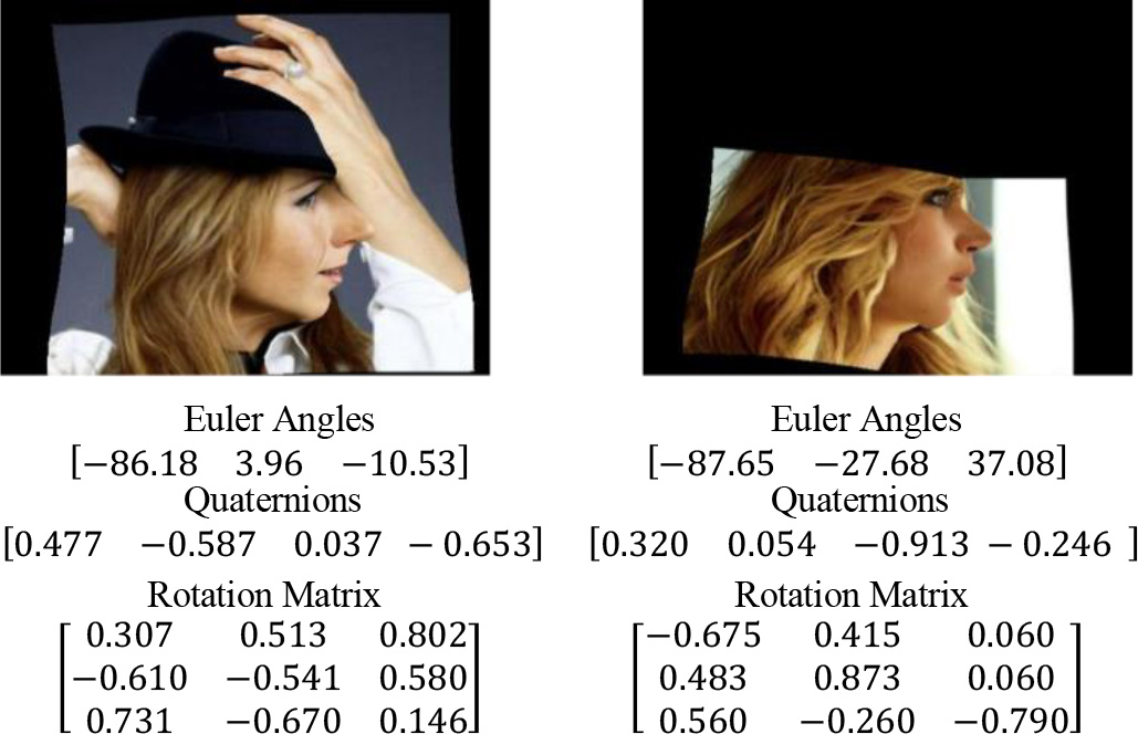
Figure 4.
Image samples from 300W-LP dataset with different rotation representations
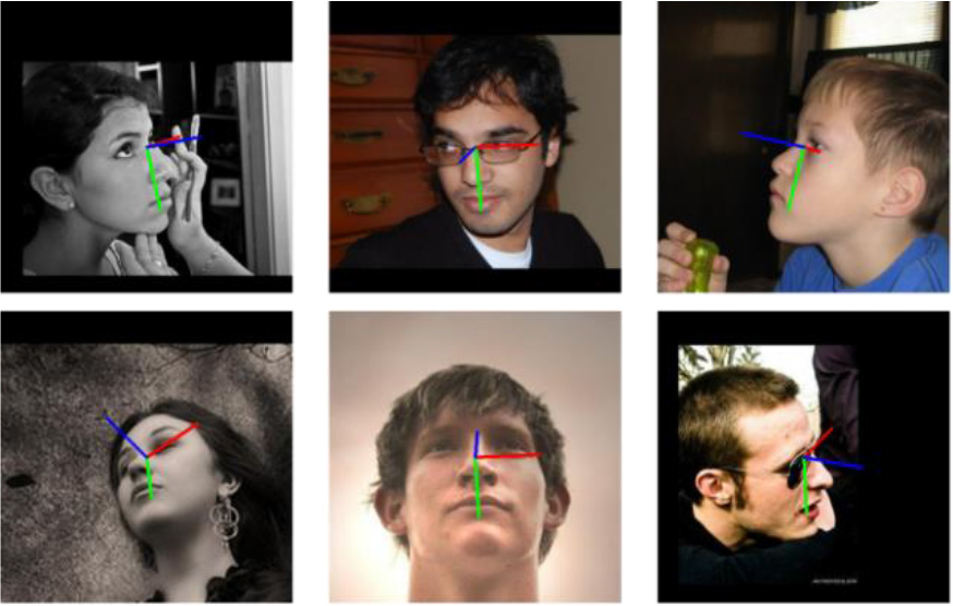
Figure 5.
Example images of Euler angle visualization using rotation matrix transformation from AFLW2000 dataset
TABLE II.
Comparisons with state-of-the-art methods on the AFLW2000 and BIWI dataset
| AFLW2000 | BIWI | |||||||
|---|---|---|---|---|---|---|---|---|
| Models | Yaw | Pitch | Roll | MAE | Yaw | Pitch | Roll | MAE |
| HopeNet[4] | 6.40 | 6.53 | 5.39 | 6.11 | 4.54 | 5.15 | 3.37 | 4.36 |
| FSA-Net[8] | 4.50 | 6.08 | 4.64 | 5.07 | 4.64 | 5.61 | 3.57 | 4.61 |
| HPE[6] | 4.80 | 6.18 | 4.87 | 5.28 | 3.12 | 5.18 | 4.57 | 4.29 |
| QuatNet[5] | 3.97 | 5.62 | 3.92 | 4.50 | 2.94 | 5.49 | 4.01 | 4.15 |
| WHENet[7] | 5.11 | 6.24 | 4.92 | 5.42 | 3.99 | 4.39 | 3.06 | 3.81 |
| TriNet[9] | 4.04 | 5.77 | 4.20 | 4.67 | 4.11 | 4.76 | 3.05 | 3.97 |
| FDN[10] | 3.78 | 5.61 | 3.88 | 4.42 | 4.52 | 4.70 | 2.56 | 3.93 |
| 6DRepNet[18] | 3.63 | 4.91 | 3.37 | 3.97 | 3.24 | 4.48 | 2.68 | 3.47 |
| 9D-EfficientNet | 3.57 | 4.69 | 3.28 | 3.85 | 4.08 | 4.17 | 2.94 | 3.73 |
TABLE IV.
Comparison of the MAE between L2 and geodesic LOSS
| AFLW2000 | BIWI | 70/30 BIWI | |
|---|---|---|---|
| Loss function | MAE | MAE | MAE |
| L2 Loss | 3.90 | 3.92 | 2.71 |
| Geodesic Loss | 3.85 | 3.73 | 2.50 |