
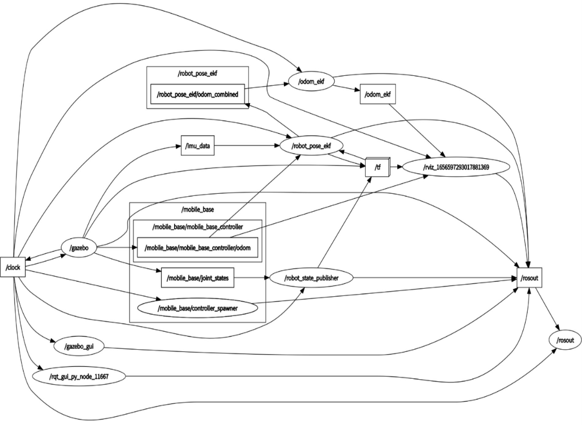
Figure 1.
Simulation fusion calculation diagram
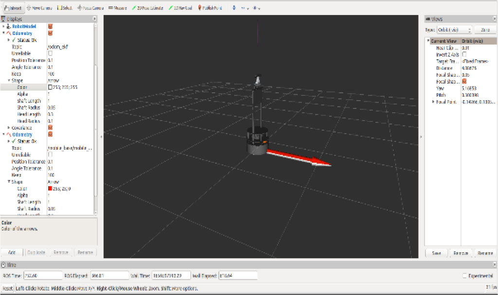
Figure 2.
Extended Kalman filter fusion results
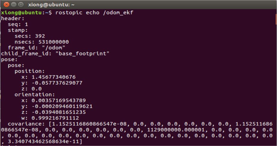
Figure 3.
Integrating odometer data
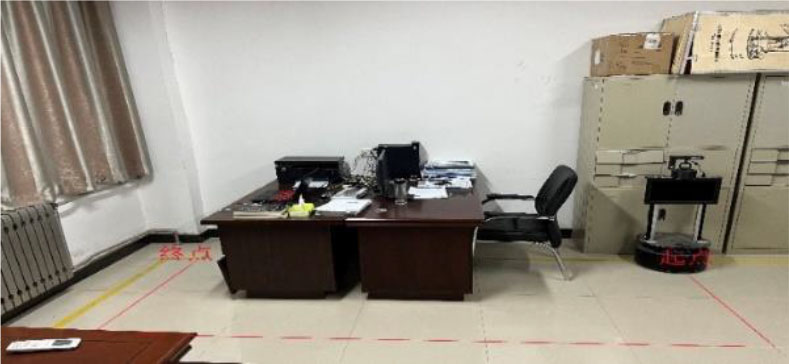
Figure 4.
Experimental scenario
TABLE I.
Experimental Result
| Starting point | Target point | Wheel odometry | Error | Fusion odometry | Error |
| (0,0) | (1.3,0) | (1.347,0.035) | (0.047,0.035) | (1.324,0.029) | (0.024, 0.029) |
| (1.3,-3.25) | (1.391,-3.373) | (0.091,0.123) | (1.386,-3.322) | (0.086, 0.072) | |
| (0,-3.25) | (0.152,-3.387) | (0.152,0.137) | (0.085,-3.316) | (0.085, 0.066) | |
| Mean error | (0.097,0.098) | (0.065, 0.056) | |||
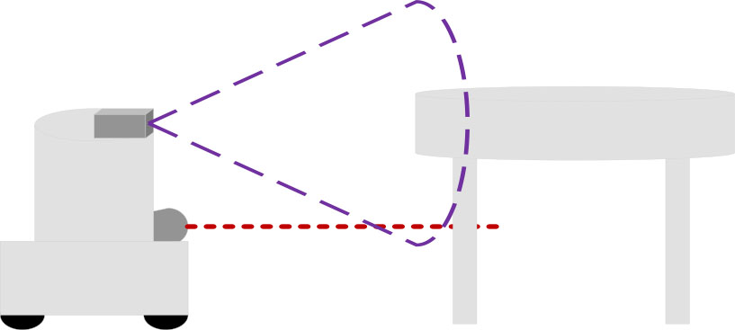
Figure 5.
Laser and visual scanning range
TABLE II.
Local map fusion rules
| 2D excitation Optical radar | Depth camera | ||
| Occupy | empty | Uncertain | |
| Occupied | Occupy | Occupy | Occupy |
| empty | Occupy | empty | empty |
| Uncertain | Occupy | empty | Uncertain |
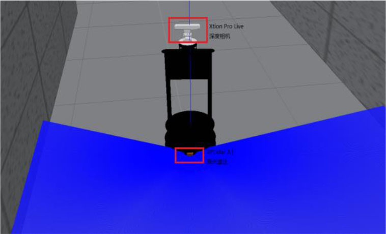
Figure 6.
Robot model
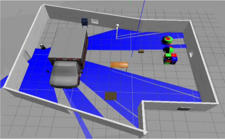
Figure 7.
Simulation experimental environment
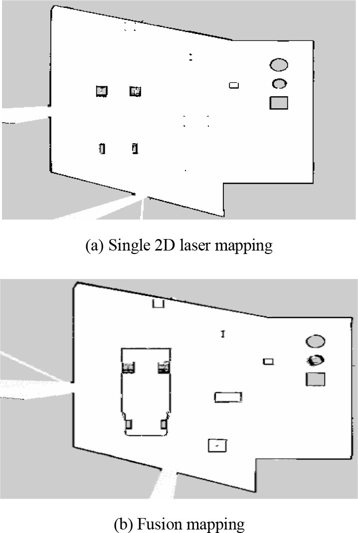
Figure 8.
Comparison of simulation experiments
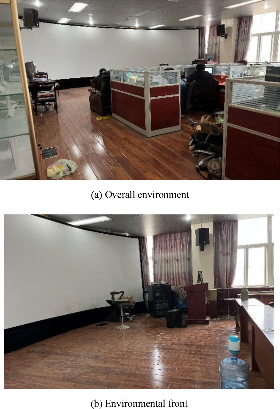
Figure 9.
Real experimental environment
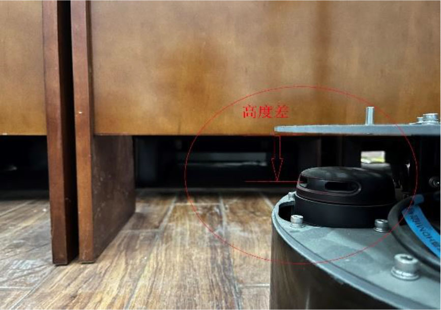
Figure 10.
Installation height of LiDAR
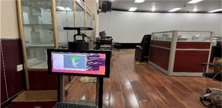
Figure 11.
Robot departure position
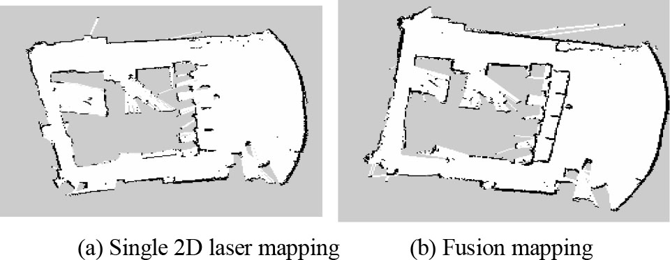
Figure 12.
Real environment mapping results
TABLE III.
Positioning results
| Actual location (m) | Actual pose (°) | Gmapping | Vision + Laser | ||||||
|---|---|---|---|---|---|---|---|---|---|
| Estimated position (m) | Estimated pose (°) | Root mean square error of position (cm) | Attitude error (°) | Estimated position (m) | Estimated pose (°) | Root Mean square error of position (cm) | Pose Error (°) | ||
| (6,0) | 30 | (6.085, 0.079) | 33.149 | 11.604 | 3.149 | (6.059, 0.037) | 31.092 | 5.9 | 1.092 |
| (6,-3) | 90 | (6.094,-3.081) | 94.634 | 12.408 | 4.634 | (6.064,-3.051) | 92.043 | 8.184 | 2.043 |
| (6,-6) | 90 | (6.103,-6.089) | 95.005 | 13.612 | 5.005 | (6.072,-6.063) | 92.729 | 9.567 | 2.729 |
| (0,-6) | 180 | (0.135,-6.112) | 186.024 | 17.541 | 6.024 | (0.089,-6.075) | 184.007 | 11.639 | 4.007 |
| (0,0) | 0 | (0.156, 0.127) | 7.678 | 20.116 | 7.678 | (0.091, 0.08) | 4.96 | 12.117 | 4.96 |