
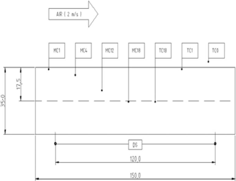
Figure 1
(a) Schematic diagram of the drying experiment and some insight into the Feutron working space of the climatic chamber (Feutron Klimasimulation GmbH, 2021).
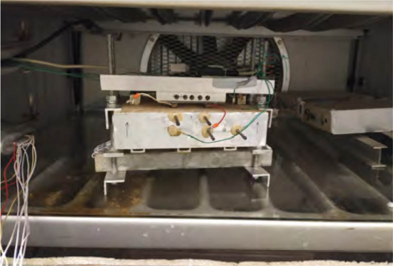
Figure 1
(b) Three specimens were used in the experiment being shown here. Sensors were attached to specimen a) to monitor the drying process; specimen b) was a reference specimen which was being used to determine the drying curve by means of weighing; and specimen c) was used to determine the moisture content of the wood at different depths by means of slicing.
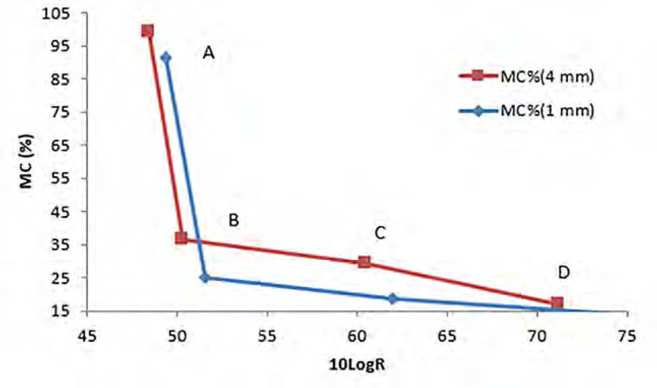
Figure 2
A cross-section linear calibration function for the calibration of resistance-type sensors into the wood's MC sensors. Points A, B, C and D are the endpoints of the line segment.
Table 1
Calibration functions were derived from Formula (4) for electrical resistance sensors at depths of 1 mm and 4 mm from the surface of the wood in sections AB, BC, and CD.
| Depth (mm) | AB | BC | CD |
|---|---|---|---|
| 1 mm | y = −30.277x+1584.9 | y = −0.6058x+56.458 | y = −0.3867x+42.873 |
| 4 mm | y = −32.895x+1691.4 | y = −0.7255x+73.292 | y = −1.1495+98.947 |
Table 2
Industrial 35 mm pine wood drying schedule used in the experiment and the simulation section.
| Time (h) | Air temp. (°C) | Air RH (%) |
|---|---|---|
| 0 | 20 | 93 |
| 1 | 47 | 93 |
| 12 | 47 | 93 |
| 36 | 50 | 90 |
| 60 | 52 | 85 |
| 84 | 52 | 80 |
| 108 | 52 | 69 |
| 132 | 52 | 59 |
| 156 | 52 | 49 |
| 180 | 52 | 39 |
| 204 | 52 | 39 |
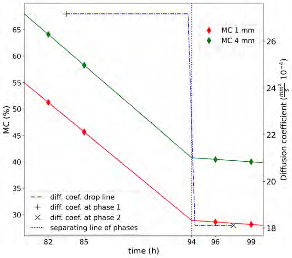
Figure 3
A schematic for calculating the diffusion coefficients in the first and second drying phases, using the four-point method based on experimental data.
Table 3
Optimized industrial pine wood drying schedule based on the definition of critical DC and critical RH.
| Time (h) | Air temp. (°C) | Air RH (%) |
|---|---|---|
| 0 | 20 | 60 |
| 1 | 47 | 83 |
| 113 | 52 | 81 |
| 132 | 52 | 59 |
| 156 | 52 | 49 |
| 180 | 52 | 39 |
| 204 | 52 | 39 |
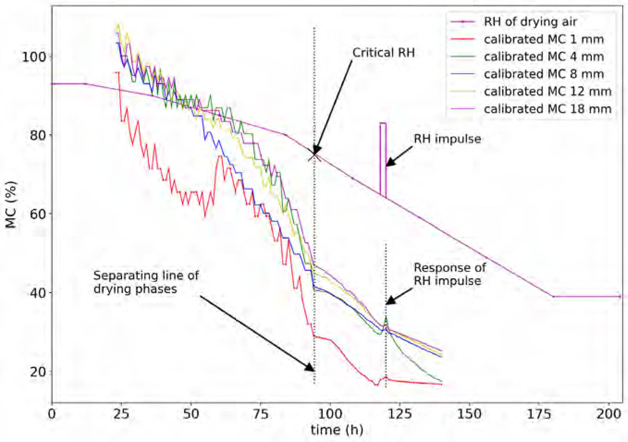
Figure 4
Identification of the critical RH of the drying air according to the separating line of the first and second drying phase.
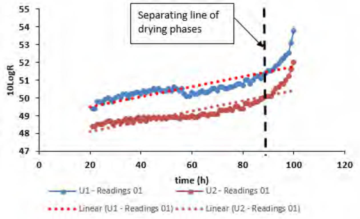
Figure 5
The response for uncalibrated electrical resistance sensors (at depths of 1 mm and 4 mm) upon transition from the first drying phase to the second drying phase.
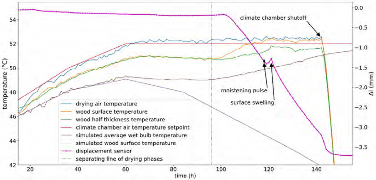
Figure 6
A distinction between the first and the second drying phases based on the log files of three Ahlborn thermocouples and an Ahlborn displacement sensor.
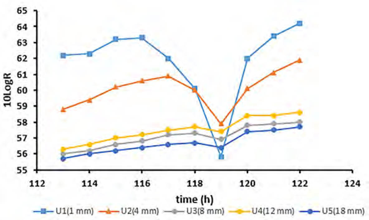
Figure 7
Effect of moistening impulse on the electrical resistance sensors.
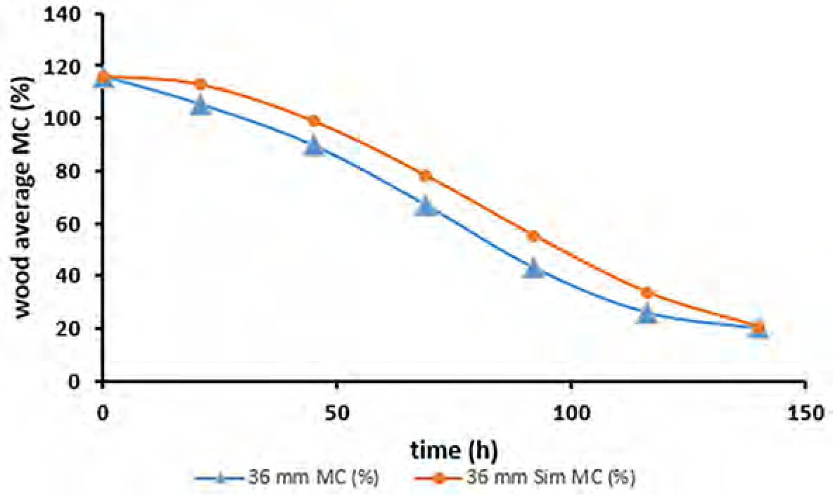
Figure 8
A comparison of drying curves under simulation and during experimentation as determined on the basis of the industrial drying schedule.
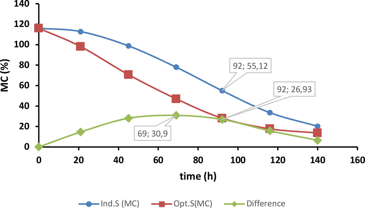
Figure 9
The results of simulations regarding optimized and unoptimized drying schedules.
Table 4
A forced drying schedule for pine wood. Data regarding the stages of the moistening impulse are given in parenthesis in the table.
| Time (h) | Air temp. (°C) | Air RH (%) |
|---|---|---|
| 0 | 20 | 93 |
| 1 | 47 | 93 |
| 24 | 47 | 77 |
| 48 | 50 | 61 |
| 72 | 52 | 45 |
| (90) | (52) | (40) |
| 96 | 52 | 29 |
| 120 | 52 | 13 |
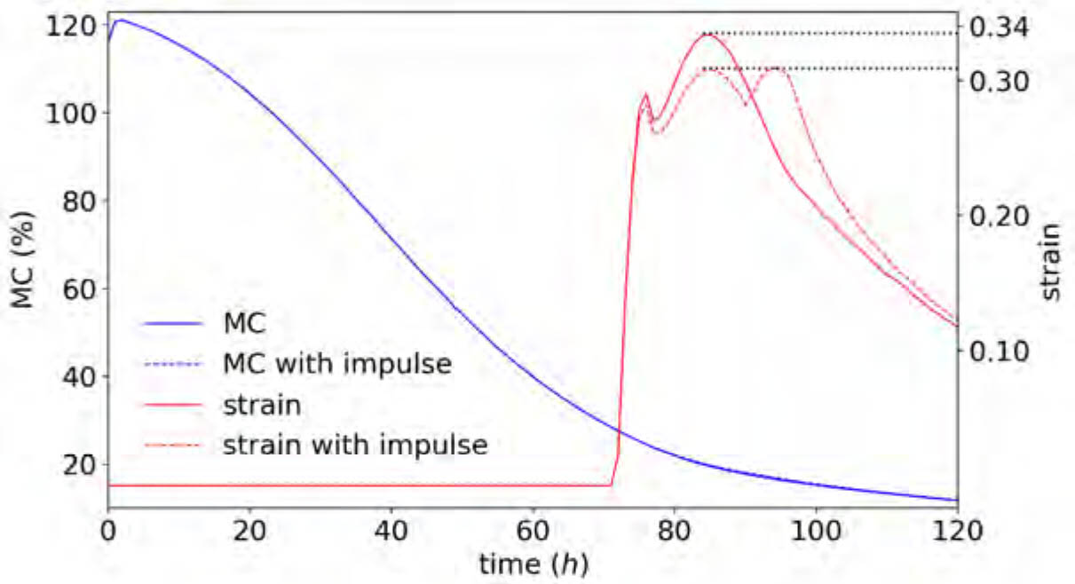
Figure 10
The forced drying schedules simulation graphs without the moistening impulse, and with the moistening impulse.
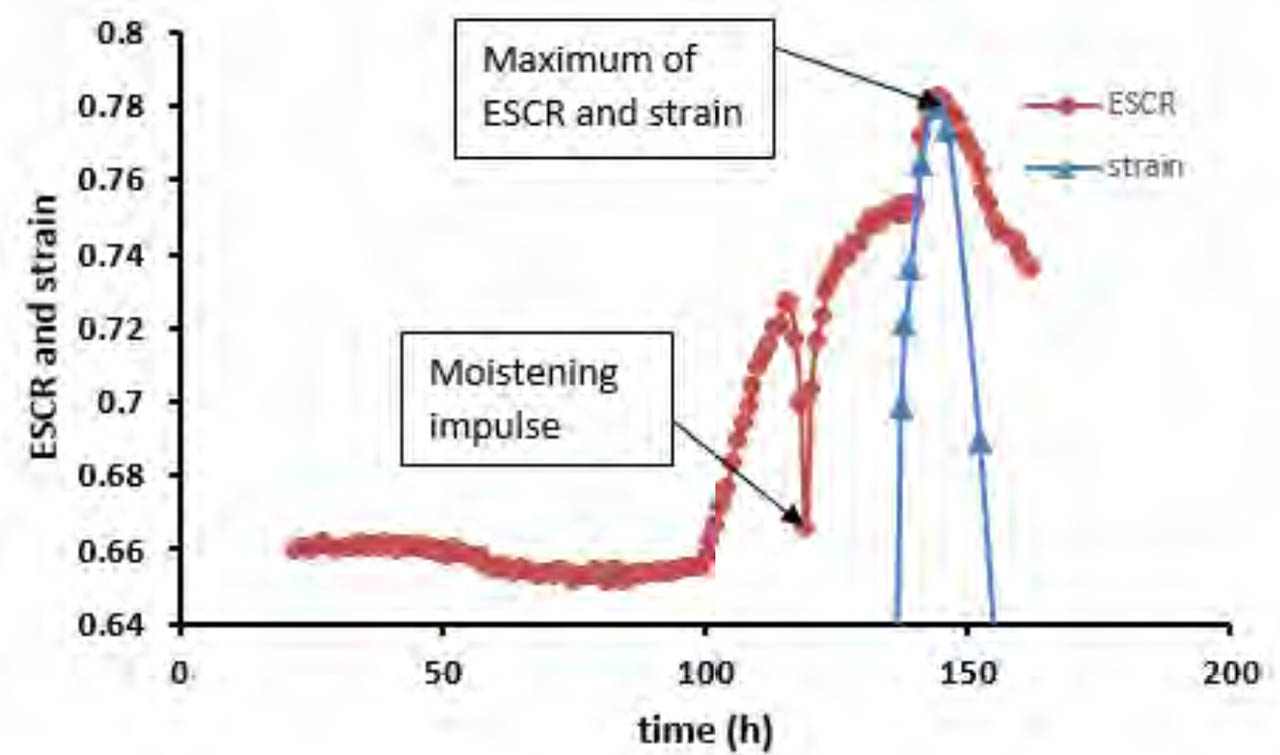
Figure 11
Dependencies of the ESCR value and the TORKSIM v5.11 simulated relative drying stresses on drying time. For a better visual comparison, the simulated relative stresses are multi plied by a factor of 3.12.
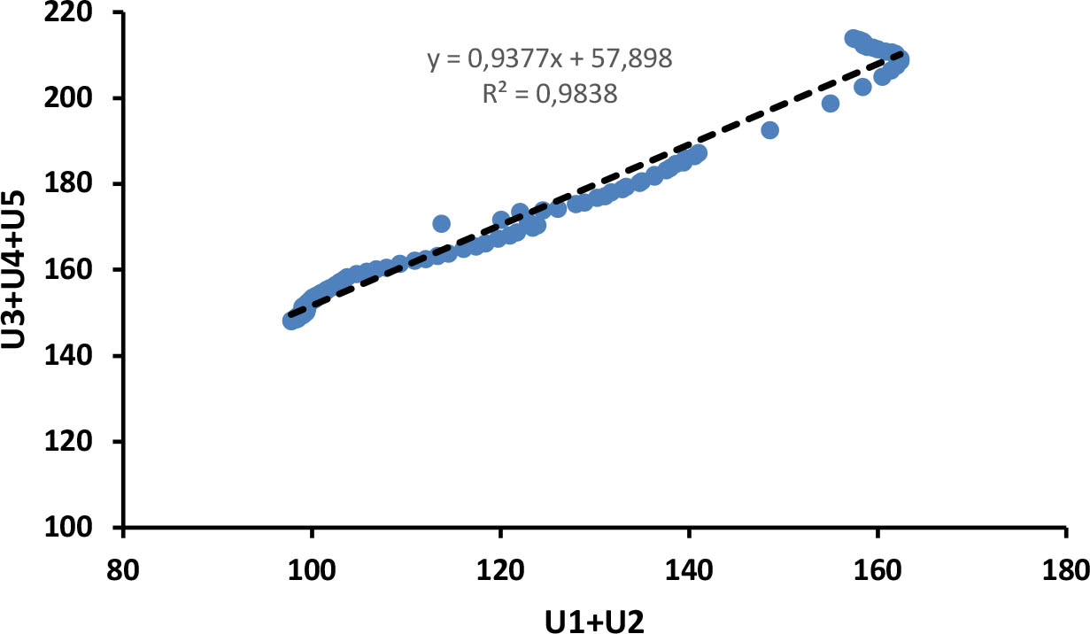
Figure 12
A linear model of the relationship between the electrical indicator for the surface layer and the electrical indicator for the inner layer.
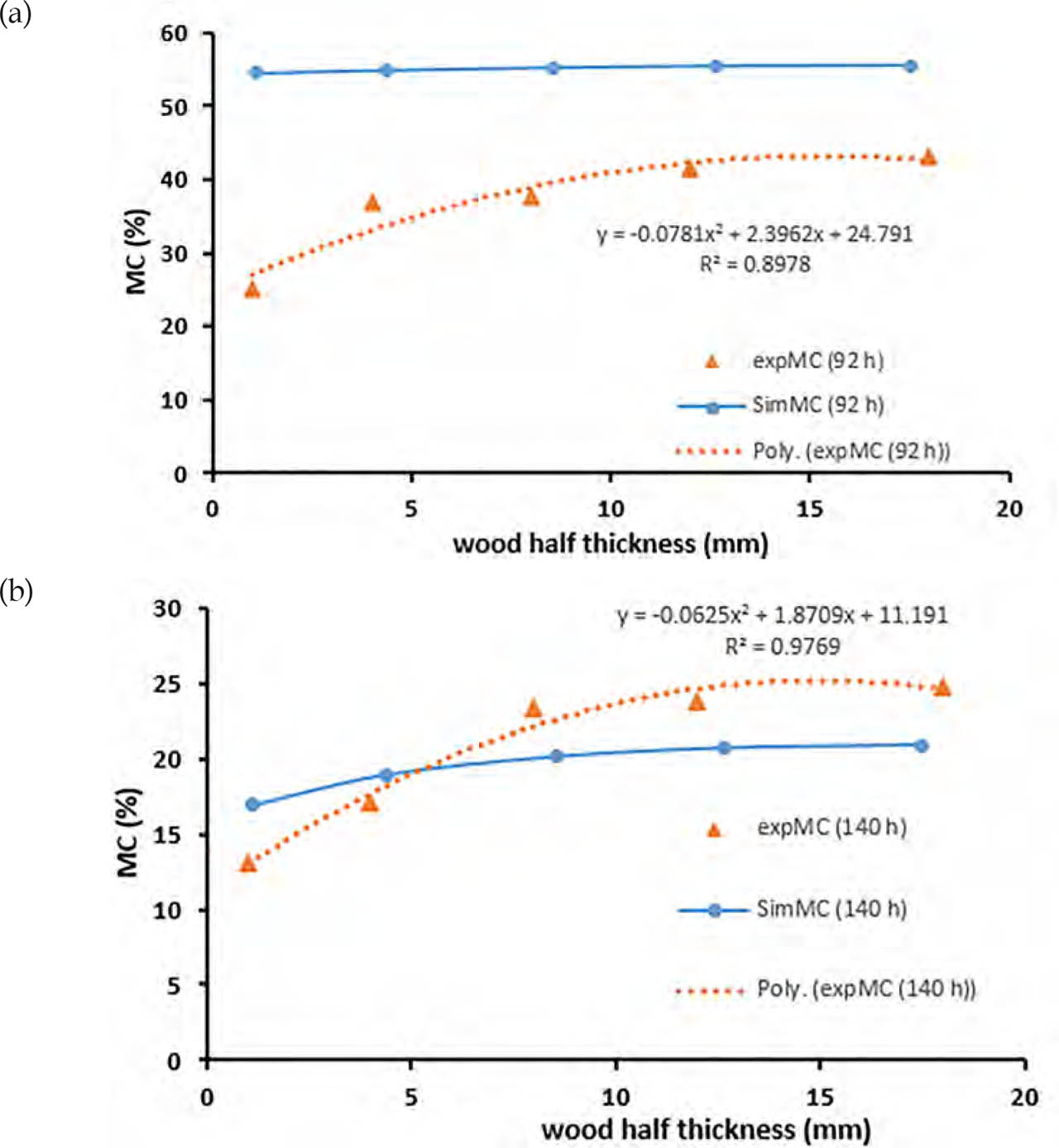
Figure 13
Comparison of experimental and simulated moisture profiles in pine wood: a) after 92 hours b) after 142 hours.