
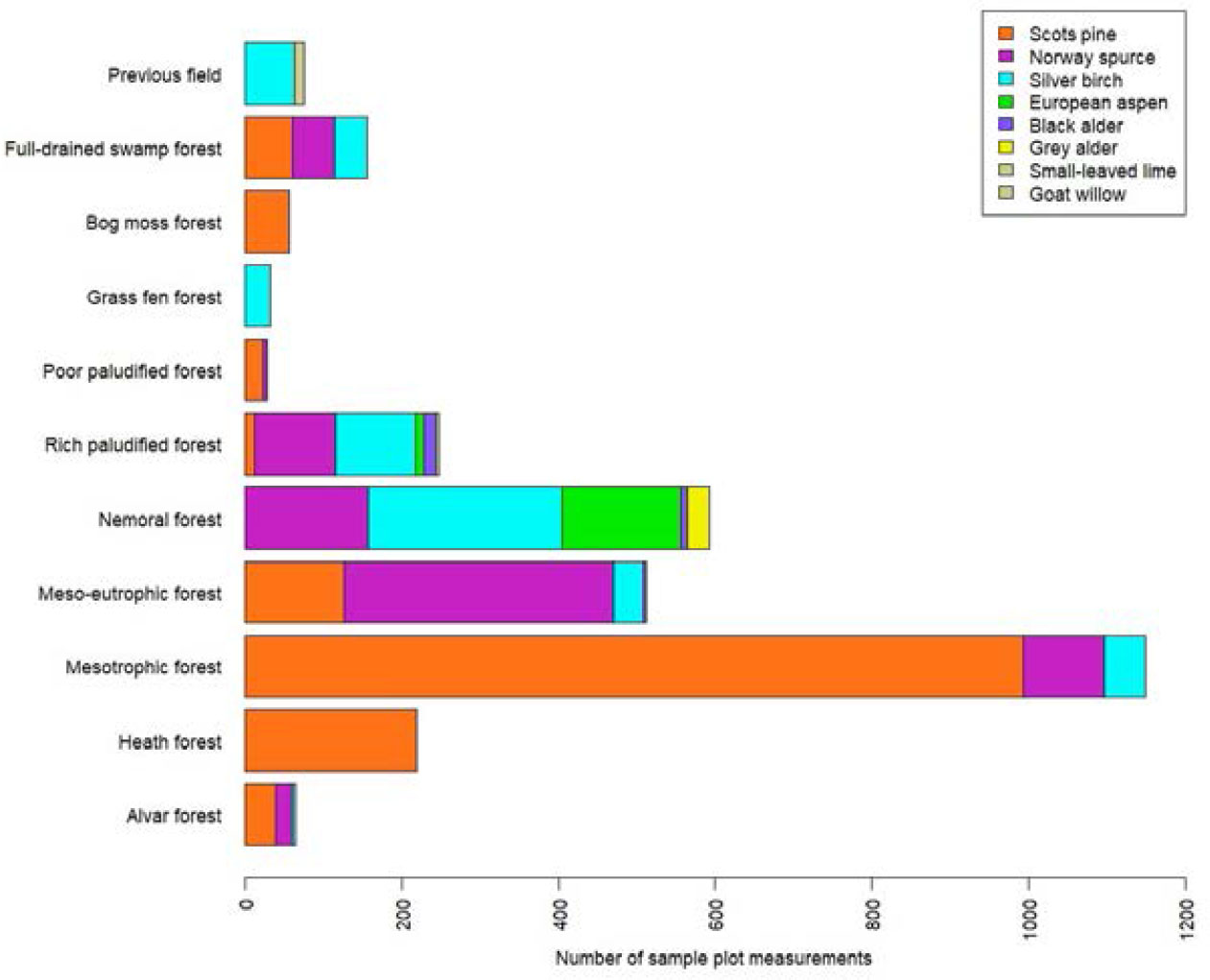
Figure 1
Distribution of the ENFRP plot measurements by forest type and main tree species.
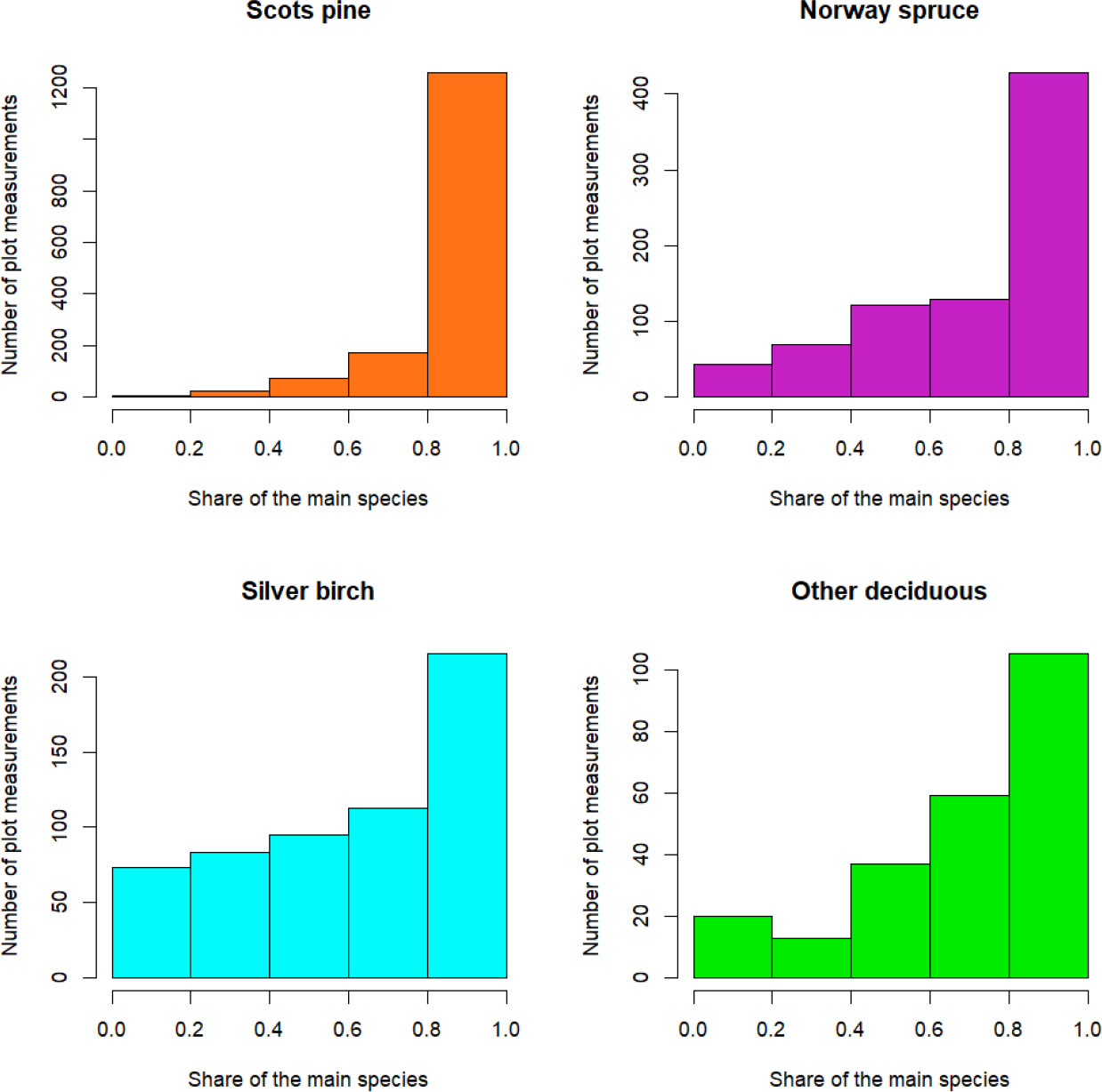
Figure 2
Distributions of the main species share in the dominant tree cohort for main species groups.
Table 1
Values of species-specific coefficients for height curve models 4, 5 and 6.
| Model | Coefficient | Scots pine | Norway spruce | Silver birch | Other deciduous |
|---|---|---|---|---|---|
| 5 | asp | 0.30201 | 0.44325 | 0.27936 | 0.27936 |
| 6 | asp | 0.32044 | 0.44103 | 0.39554 | 0.25803 |
| 6 | bsp | 0.00434 | 0.00643 | 0.00629 | 0.00582 |
| 4, 6 | csp | 1.48076 | 1.37255 | 1.32998 | 2.04430 |
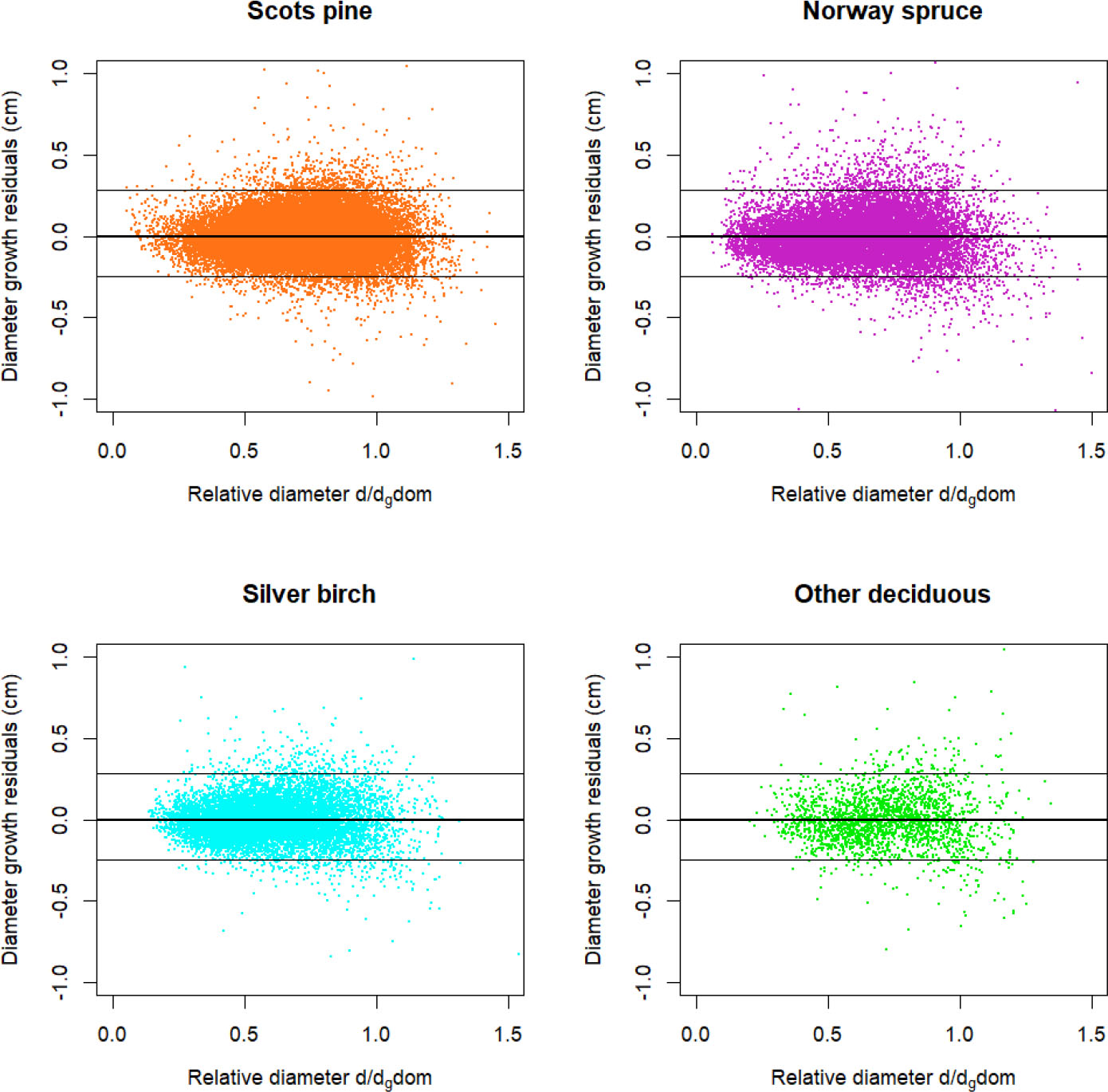
Figure 3
Distribution of residuals and threshold values for excluding diameter annual increment (id) outliers on a scatterplot of id mixed model residuals and relative diameter (d/dgdom).
Table 2
Fit statistics of the height curve models (2–6) for dominant trees based on experimental data. (n – number of trees; me – mean residual; sde – mean square residual; p-value – p-value of t-test; desc – number cohorts with a descending height curve).
| Statistic | Scots pine | Norway spruce | Silver Birch | Other deciduous | All species |
|---|---|---|---|---|---|
| n | 5165 | 914 | 426 | 76 | 6581 |
| Model (2) me | −0.08 | −0.17 | −0.18 | −0.23 | −0.10 |
| Model (2) sde | 1.37 | 1.18 | 1.38 | 1.41 | 1.35 |
| Model (2) p-value | <0.001 | <0.001 | 0.008 | 0.165 | <0.001 |
| Model (2) desc | 5 | 0 | 1 | 0 | 6 |
| Model (3) me | −0.07 | −0.13 | −0.15 | −0.21 | −0.09 |
| Model (3) sde | 1.37 | 1.18 | 1.38 | 1.40 | 1.35 |
| Model (3) p-value | <0.001 | 0.001 | 0.025 | 0.188 | <0.001 |
| Model (3) desc | 5 | 0 | 1 | 0 | 6 |
| Model (4) me | −0.01 | −0.08 | −0.11 | 0.01 | −0.03 |
| Model (4) sde | 1.37 | 1.17 | 1.37 | 1.35 | 1.34 |
| Model (4) p-value | 0.602 | 0.044 | 0.113 | 0.937 | 0.127 |
| Model (4) desc | 5 | 0 | 1 | 0 | 6 |
| Model (5) me | −0.09 | −0.61 | −0.14 | −0.44 | −0.17 |
| Model (5) sde | 1.47 | 1.45 | 1.51 | 1.49 | 1.47 |
| Model (5) p-value | <0.001 | <0.001 | 0,060 | 0,009 | <0.001 |
| Model (6) me | −0.03 | −0.05 | −0.23 | 0.02 | −0.04 |
| Model (6) sde | 1.47 | 1.32 | 1.52 | 1.37 | 1.45 |
| Model (6) p-value | 0.142 | 0.301 | 0.002 | 0.896 | 0.013 |
Table 3
Height curve statistics specifications for Table 2.
| Height curve statistics |
|---|
| n – number on dominant trees; |
| me – arithmetic mean residual hmeasured – hpredicted (systematic error); |
| sde – quadratic mean residual hmeasured – hpredicted (random error); |
| p-value – t-test for hypothesis that mean residual is different from zero; |
| desc – despite excluding outliers and a moderate number of observations (n ≥ 16) in each cohort, the height curve was descending (parameter a < 0 for models 2 and 3, parameter b < 0 for model 4) in the case of some cohorts. |
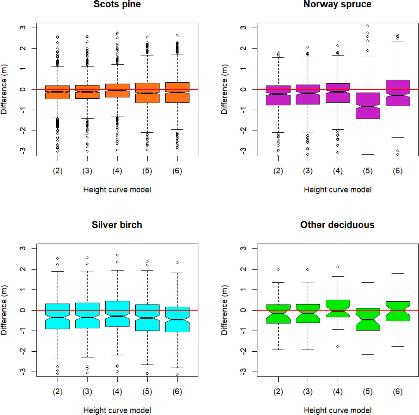
Figure 4
The difference between the estimated dominant height hgdom and the empirical arithmetic mean height of the 100 thickest trees per hectare.
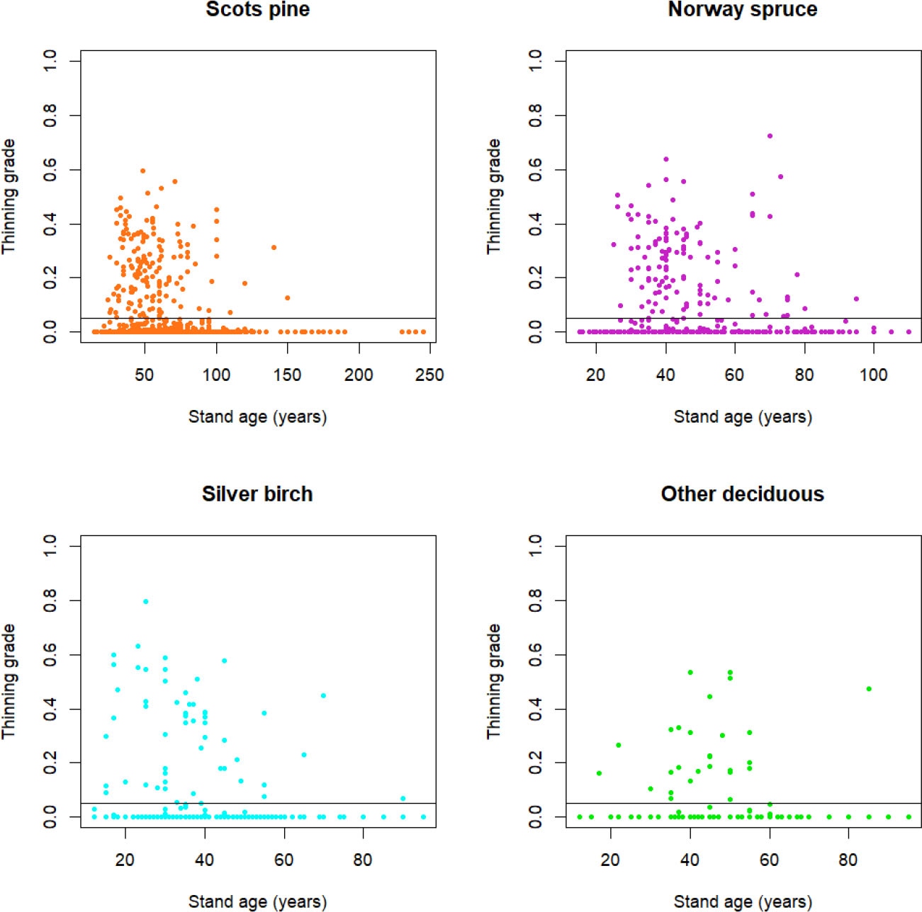
Figure 5
Share of the thinned basal area in the basal area of the main species between two consecutive plot measurements depending on stand age. The solid horizontal line shows a 5% threshold value for thinning.
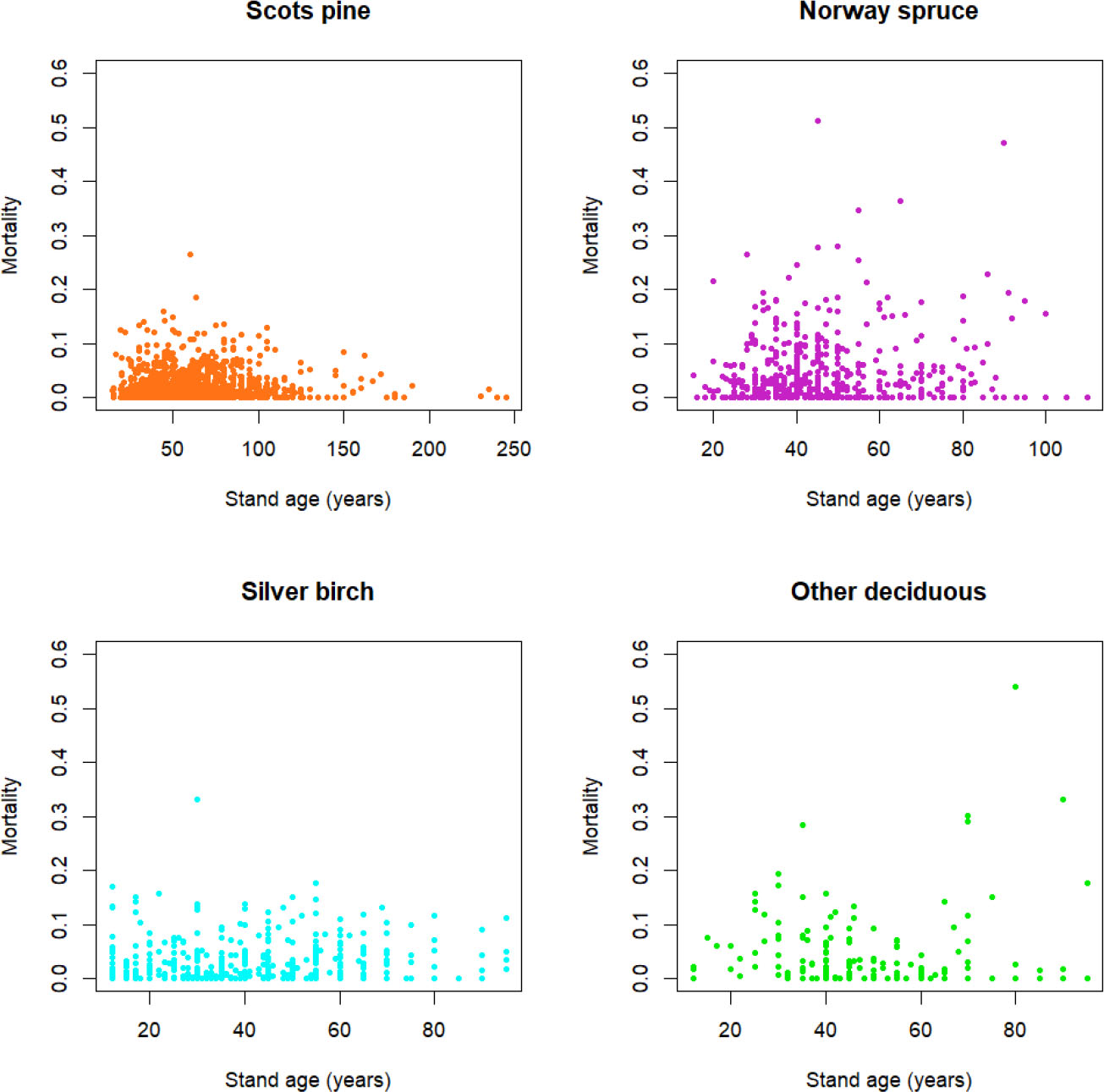
Figure 6
The share of the dead tree basal area in the basal area of the main species between two consecutive plot measurements depending on stand age.
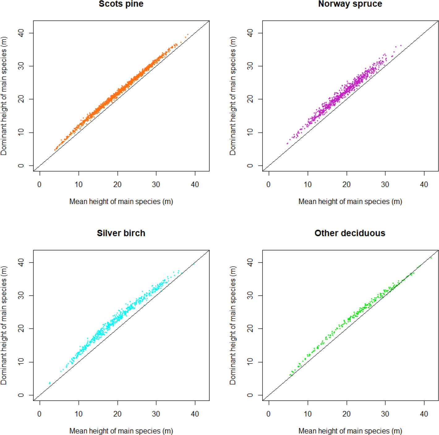
Figure 7
Scatterplots of the mean height hg and the dominant height hgdom of cohorts by tree species.
Table 4
Species-specific coefficients for regression model (9).
| Coefficient | Scots pine | Norway spruce | Silver birch | Other deciduous |
|---|---|---|---|---|
| a0 | 2.0494 | 3.3661 | 3.0474 | 1.7910 |
| a1 | −0.0964 | −0.1231 | −0.0824 | −0.1108 |
| a2 | −15.686 | −14.070 | −34.854 | −15.215 |
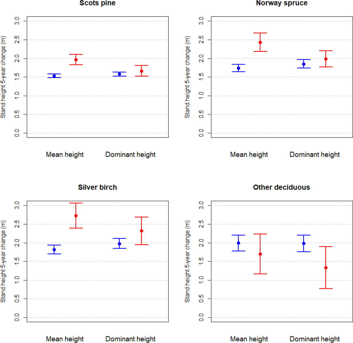
Figure 8
The average change in the mean height and dominant height with a 95% confidence interval. The sample plots were measured at a 5-year interval. Red dots represent thinned sample plots and blue dots represent unthinned sample plots.
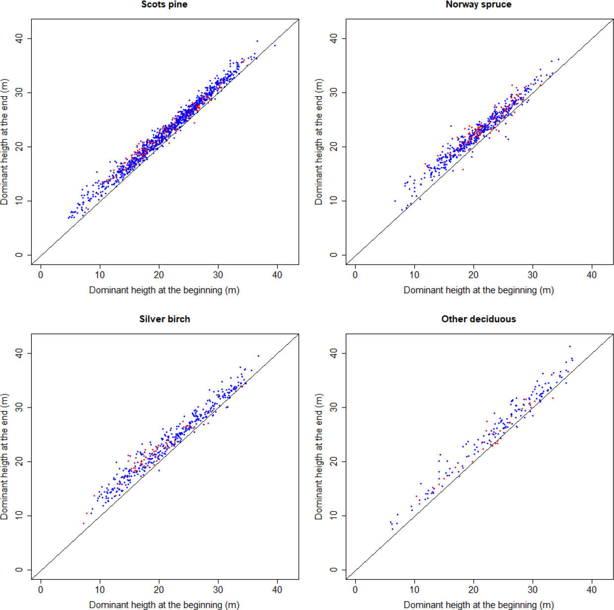
Figure 9
The difference in the dominant height between the beginning and the end of the five-year period. Red dots represent thinned sample plots and blue dots represent unthinned sample plots.
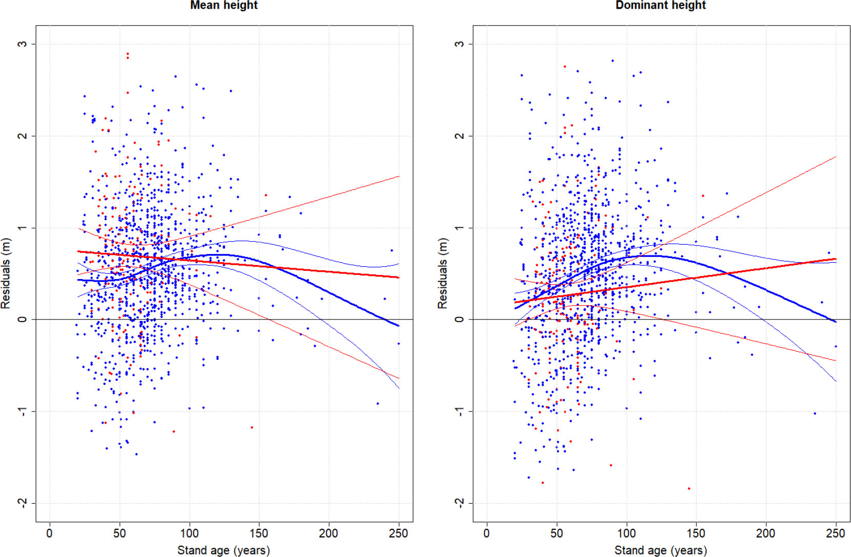
Figure 10
Growth error of the mean height model (7) and the dominant height model (8). Red dots represent thinned sample plots and blue dots represent unthinned sample plots.