
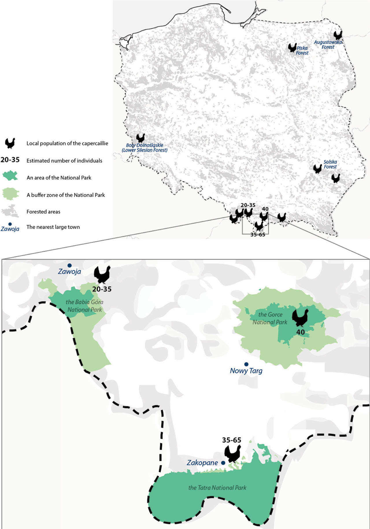
Figure 1.
Map of the distribution of the capercaillie in Poland, with particular emphasis on the Carpathian subpopulations covered by this study. The estimated number of individuals was based on data from the work of Zawadzka et al. (2019)
Table 1.
Information about the collected biological material and basic measures of genetic diversity, determined on the basis of polymorphism of 9 microsatellite loci.
| GOR | TAT | BAB | GORT | TATT | BABT | Total | ||||
|---|---|---|---|---|---|---|---|---|---|---|
| GOld | GNew | TOld | TNew | BOld | BNew | Both periods | ||||
| Ncol | 346 | 156 | 221 | 179 | 204 | 200 | 520 | 400 | 404 | 1324 |
| Nsuc | 227 | 102 | 117 | 99 | 127 | 117 | 329 | 216 | 244 | 789 |
| Nind | 44 | 21 | 28 | 39 | 35 | 29 | 64 | 66 | 64 | 194 |
| Na | 3.89 | 3.78 | 5.56 | 5.22 | 4.78 | 5.33 | 4.33 | 5.67 | 5.78 | 6.55 |
| R | 3.77 | 3.78 | 5.55 | 4.91 | 4.66 | 5.05 | 3.73 | 5.14 | 4.76 | – |
| Pa | 0.111 | 0.111 | 1.111 | 0.444 | 0.333 | 0.333 | 0.111 | 0.565 | 0.565 | – |
| Ho | 0.593 | 0.608 | 0.671 | 0.641 | 0.578 | 0.617 | 0.598 | 0.653 | 0.595 | 0.616 |
| He | 0.583 | 0.591 | 0.669 | 0.629 | 0.616 | 0.660 | 0.590 | 0.653 | 0.649 | 0.654 |
| HWE | 0.009 | 0.052 | 0.445 | 0.068 | 0.132 | 0.303 | <0.001 | 0.003 | <0.001 | <0.001 |
| Fis | −0.007 | −0.005 | 0.015 | −0.006 | 0.077 | 0.083 | −0.005 | 0.007 | 0.090 | 0.060* |
GOR – The Gorce National Park; TAT – The Tatra National Park; BAB – Babia Góra National Park; GORT – total data (for both study periods) about the Gorce National Park; TATT – total data (for both study periods) about the Tatra National Park; BABT – total data (for both study periods) about Babia Góra National Park; GOld – data for 2010–2013 about the Gorce National Park; GNew – data for 2021–2022 about the Gorce National Park; TOld – data for 2010–2013 about the Tatra National Park; TNew – data for 2021–2022 about the Tatra National Park; BOld – data for 2010–2013 about Babia Góra National Park; BNew – data for 2021–2022 about the Babia Góra National Park; Ncol – number of samples collected; Nsuc – number of samples successfully analysed (reliable genotype was obtained); Nind – number of unique genotypes identified, hence corresponding to the number of identified individuals; Na – number of alleles; R – allelic richness; Pa – number of private alleles; Ho – observed heterozygosity; He – expected heterozygosity; HWE – the results of HWE exact test for heterozygote deficiency/excess (P-value was given); Fis – inbreeding coefficient;
Table 2.
Among-population genetic differentiation based on pairwise Fst sensu Weir and Cockerham [1984]. All Fst values are significant after Bonferroni correction, except of values shown in dark grey. Abbreviation of comparing groups of samples as in Table 1
| GOld | TNew | TOld | BNew | BOld | |
|---|---|---|---|---|---|
| GNew | 0.0013 | 0.0435 | 0.0557 | 0.0794 | 0.0843 |
| GOld | 0.0372 | 0.0515 | 0.0631 | 0.0672 | |
| TNew | 0.0083 | 0.0415 | 0.0383 | ||
| TOld | 0.0258 | 0.0211 | |||
| BNew | 0.0229 | ||||
| GORT | TATT | ||||
| TATT | 0.0426 | ||||
| BABT | 0.0647 | 0.0251 |
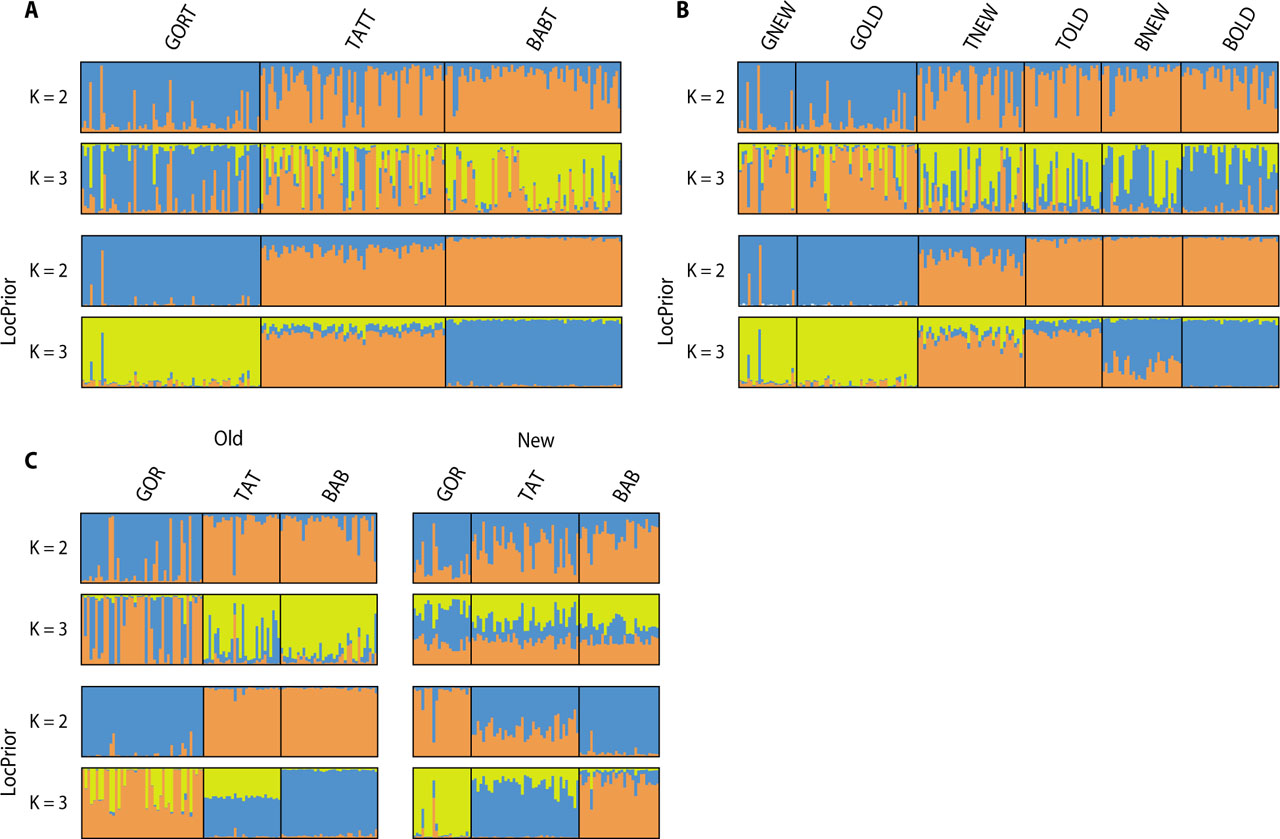
Figure 2.
Results of analysis in STRUCTURE. In bar plots each individual is represented by a vertical bar partitioned into segments. The length of each segment describes the estimated membership proportions to each of the genetic clusters. Although ΔK suggested division into two clusters, the bar plot for K = 3 (corresponding to the number of geographical groups) was also presented. Abbreviations of groups (subpopulations) as in Table 1. A – results of analysis in STRUCTURE based on total (cumulative for both periods) number of unique genotypes in each subpopulation; B - results of analysis in STRUCTURE based on unique genotypes from both periods independently in 3 subpopulations; C – results of analysis in STRUCTURE based on unique genotypes identified independently for each period in each subpopulation
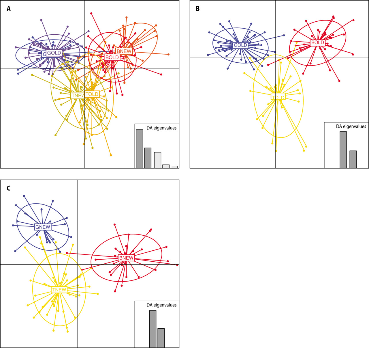
Figure 3.
Results of DAPC analysis. DAPCs are shown for the first (x-axis) and the second (y-axis) discriminant function. Abbreviations of groups (subpopulations) as in Table 1. A – results of DAPC analysis based on unique genotypes in each subpopulation in each period; B – results of DAPC analysis based on unique genotypes identified in 2010–2013; C – results of DAPC analysis based on unique genotypes identified in 2021–2022