
Figure 1
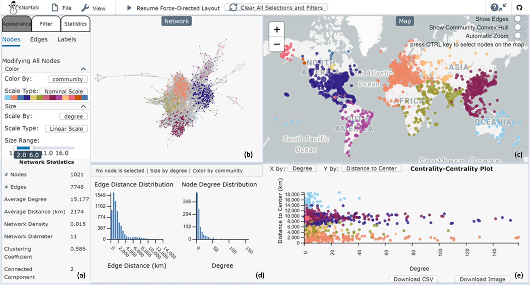
The SNoMaN interface, showing a world flight network of 1,022 airports (i.e., nodes) and 7,748 direct flights (i.e., edges) (OurAirport, 2017). It is subdivided into different elements: (a) is the network statistics panel, (b) is a force directed sociogram, (c) is a map where nodes in the sociogram are mapped, (d) is a panel containing two histograms, and (e) contains a scatterplot. All elements are linked and respond to brushing and filtering.
Source: data from: OurAirport. (2017). Airport, Airline and Route Data. Retrieved from https://ourairports.com/data/.
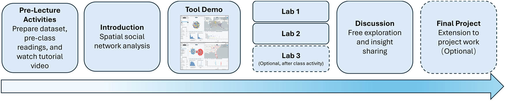
Figure 2
Course module timeline showing the instructional flow, including a preclass activity, module introduction, tool demonstration, three in-class lab exercises, a guided discussion, and an optional extension into the final project.
Source: Authors’ contribution.
Table 1
Structure of the SNoMaN lab modules and covered sections.
| Lab 1 – Visualization Configurations and Interaction |
| Import dataset |
| Customize and interact with networks; compute network statistics |
| Visualize weighted or directed networks; identify important nodes |
| Compute statistics for selected subnetworks |
| Lab 2 – Correlation Analysis on Geographic Impact on Connectivity at Node, Path, and Community Levels |
| Node-level correlation analysis (network centrality vs location) Path-level correlation analysis (network vs geographic distance) Community-level correlation analysis |
| Detecting network communities and mapping results; visualizing community spatial expanse using convex hulls; comparing network density with spatial dispersion and size |
| Lab 3 – Advanced Statistics and Metrics on Geographic Segregation and Connectivity Efficiency |
| K-fulfillment (local connection/disconnection) |
| Flattening ratio (overall spatial tightness) |
| Data assortativity function (degree correlation) |
| Average nearest neighbor plots (community clustering) |
Source: Authors’ contribution.
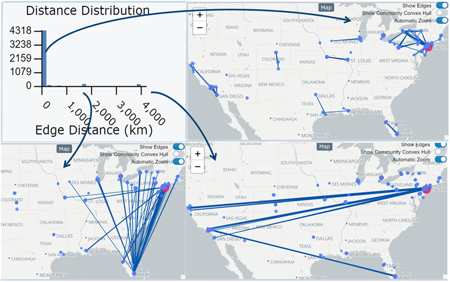
Figure 3
The distance distribution of the mafia social network (nodes represent Mafia members and edges represent criminal associations) (Andris et al., 2021) shows that connection frequency decreases as the geographic distance between members increases, illustrating the distance decay effect. By examining different distance ranges, we can see that most connections are local, with some long-distance connections between Miami and the Northeastern region, and a few rare connections spanning the East and West coasts.
Source: data from: Andris, C., DellaPosta, D., Freelin, B. N., Zhu, X., Hinger, B., & Chen, H. (2021). To racketeer among neighbors: Spatial features of criminal collaboration in the american mafia. International Journal Of Geographical Information Science, 35(12), 2463–2488. Retrieved from https://doi.org/10.1080/13658816.2021.1884869.
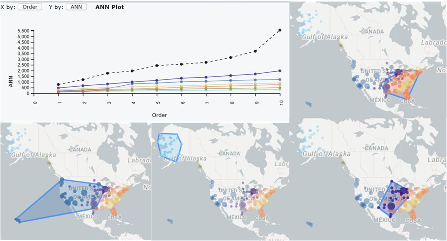
Figure 4
Example of examining geographic segregation of communities in a flight network (OurAirport, 2017) from the module. Convex hulls outline the service areas of detected communities. The Average Nearest Neighbor plot shows which communities (by color) are more or less clustered than expected (shown by position below or above a dashed line, respectively) under random community assignment.
Source: data from: OurAirport. (2017). Airport, Airline and Route Data. aRetrieved from https://ourairports.com/data/.
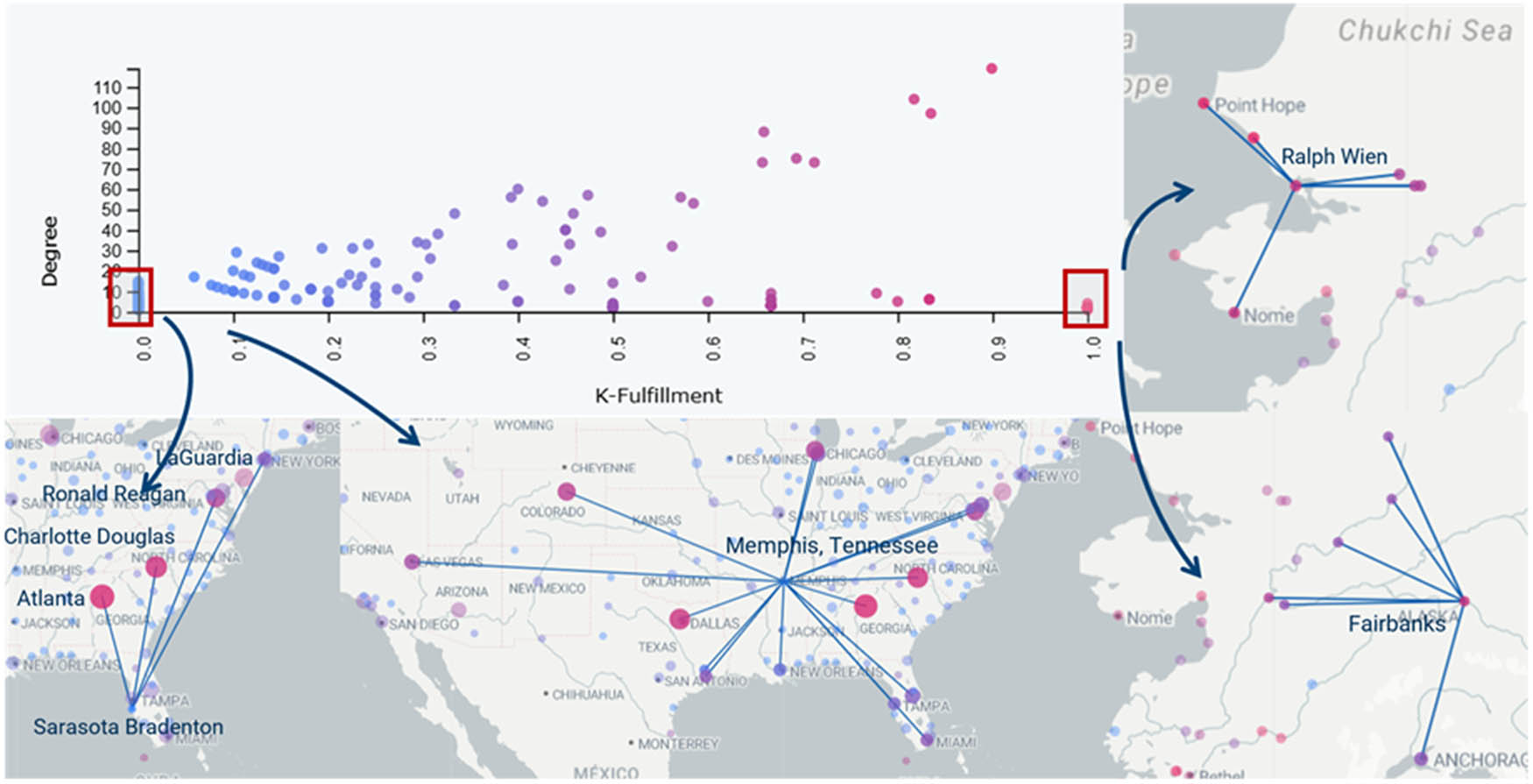
Figure 5
An example in the flight network showing that airports with high K-fulfillment scores are primarily connected to nearby airports, whereas airports with a score of zero have none of their connections to the closest airport.
Source: data from: OurAirport. (2017). Airport, Airline and Route Data. aRetrieved from https://ourairports.com/data/.
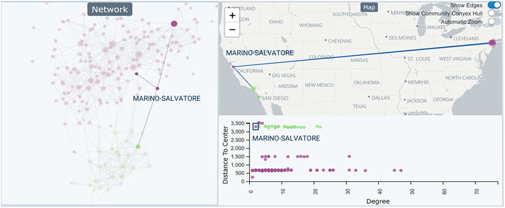
Figure 6
In the Mafia network, Salvatore Marino is identified from the force-directed layout as a bridge between two families. Selecting this node highlights its geographic location on the map: it is far from its own family base but close to the other family it connects to, suggesting a potential remote agency role.
Source: data from: Andris, C., DellaPosta, D., Freelin, B. N., Zhu, X., Hinger, B., & Chen, H. (2021). To racketeer among neighbors: Spatial features of criminal collaboration in the american mafia. International Journal Of Geographical Information Science, 35(12), 2463–2488. Retrieved from https://doi.org/10.1080/13658816.2021.1884869.
Table 2
Courses using SNoMaN teaching module across universities (ordered by first survey return date to last date).
| University | Course number & title | Department | Class size | Student level | Labs used |
|---|---|---|---|---|---|
| University of Michigan | URP 538, UT 438, URP 610 Urban Networks | Urban Planning | 15–20 | Undergraduate & Graduate | Labs 1 &2 |
| Carleton University | GEOM 3005 Geospatial Analysis | Geography | 25 | Undergraduate | Labs 1–3 |
| University of Colorado, Colorado Springs | GES 4070/GES 5070 Geovisualization | Geography & Environmental Studies | 24 | Undergraduate& Graduate | Labs 1 &2 |
| National Autonomous University of Mexico | 74236 Network Analysis in Human Geography | Geography | 7 | Graduate | Not formally completed |
| Georgia Institute of Technology | CS/CP 8803 Interactive Maps & Geovisualization | Urban Planning and Computer Science | 10–22 | Graduate | Labs 1 & 2 |
| University College Dublin | IS 41510 Social Networks Online and Offline | Information and Communication Studies | 35 | Graduate | Labs 1–3 |
| University of Florida | GIS 4113/GIS 6104 Spatial Networks | Geography | 20–25 | Undergraduate & Graduate | Labs 1 & 2 |
| Northern Illinois University | Honors 310 The Making of Modern Science: Natural History, Philosophy and Technology | University Honors Program/Division of Academic Affairs | 19 | Undergraduate | Labs 1–3 (in progress) |
Source: Authors’ contribution.
Table 3
Synthesis of instructor feedback by evaluation aspects.
| Evaluation aspects | Findings | Major consensus | Additional findings |
|---|---|---|---|
| Student learning experiences and outcomes | Student difficulties observed | Conceptual confusion between geographic and network concepts was common | Specific barriers included confusion between geographic and network distance (n = 3); understanding community detection (n = 1); translating lab questions into network metrics (n = 1); understanding terms (n = 2); geographic coordinate notation (n = 1); language barriers (n = 1) |
| Student performance | Students generally performed well on basic visualization and interaction steps (n = 3) | Struggles included interpreting advanced metrics (assortative mixing, flattening ratios, betweenness) (n = 1); shortest path in disconnected networks (n = 1); correlation interpretation (n = 1); GIS/SNA core concepts (n = 1); certain Lab 1 and 2 questions (n = 1); some classes were still in progress (n = 3). | |
| Learning curve | No activities or labs were described as “hard” | Tool or labs described as easy (n = 3); moderate for tool/metrics (n = 4 contexts); moderate-to-hard for CS students (n = 1); one course did not formally complete labs (n = 1) | |
| Student takeaways | Only three instructors reported clear takeaways | Students noted networks and geography can mix (n = 1); found SNo-MaN fun and intuitive (n = 1); applied learning to thesis and publication (n = 1); observed geographic influence on network disconnections (n = 1); three courses were in progress | |
| Instructional reflections and course design | Lab modifications | Four instructors reported no major structural changes | One instructor divided the labs into smaller pieces for timing; another collated all three labs into a single assignment and removed steps to allow exploration |
| Proposed instructional adjustments | Timing adjustments were a recurring theme | Introduce earlier (n = 1); introduce later (n = 1); pair students for discussion (n = 1); move to advanced GIS course and follow with R (n = 1); two 75-minute sessions instead of one (n = 1) | |
| Learning objectives using SNoMaN | Geovisualization and network analysis were common objectives (n = 4) | Three instructors emphasized understanding network–geography interplay; one highlighted software design–oriented learning | |
| Alternative teaching approach | Instructors would still teach spatial social networks without SNoMaN (n = 4) | Alternatives included Flowmapper, R with igraph, Python with Net-workX; two instructors would remove SSN modules | |
| Future applications and improvements | Future use | Seven of eight instructors indicated future use | One instructor did not use it in 2025 due to lack of student preparedness but may adopt it in the future if GIS prerequisites improve |
| Suggested improvements | Improve lab clarity and expand support features | Clearer wording (n = 1); more open-ended questions (n = 1); additional built-in datasets (n = 1); more theoretical resources (n = 1); improved map functionality (n = 1); multilingual versions (n = 1); alternative questions for varied backgrounds (n = 1) |
Source: Authors’ contribution.
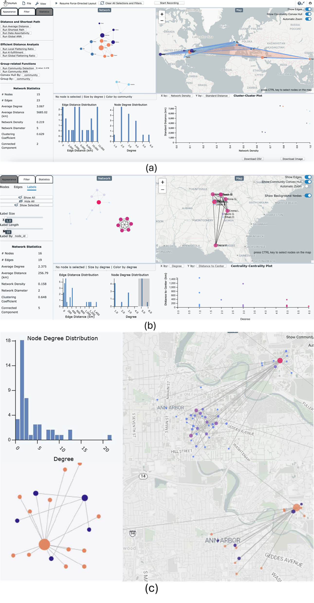
Figure 7
Screenshots of SNoMaN provided by students who used the software outside of the three written labs (for an in-class project on personal friendship networks (a and b) and an open-ended final project (c).
Source: Authors’ contribution.