

1. Introduction
Research on the historical performance and volatility of the Euro Stoxx 50 has recently become a significant topic among researchers due to its central role in European equity markets and its implications for portfolio risk management and asset allocation, which are integral to the global financial system (Batten et al., 2023). The evolution of volatility modelling has developed to advanced econometric frameworks such as generalised conditional heteroskedasticity (GARCH) and Markov-switching models, reflecting the growing sophistication of dynamics in capturing time-varying risk (De la Torre-Torres, Galeana-Figueroa & Álvarez-García, 2021; Stamos & Zimmerer, 2021; Batten et al., 2023; Caporale, Rubio-Bezares & Gil-Alana, 2024).
To remain resilient during turbulent market conditions while capitalising on opportunities presented by volatility, the need for more active development in volatility management is obvious. Unlike static portfolio strategies that maintain fixed allocations regardless of market changes, active management offers a more responsive approach, minimising downside risk and stabilising returns over the long term. However, practical challenges persist in implementing active volatility strategies (Ruslaini, Muhammad & Nurhasanah, 2025).
Volatility management can mitigate the adverse effects of extreme market fluctuations, particularly during periods of uncertainty. While high volatility is traditionally seen as a signal of increased risk, the right strategy can exploit these fluctuations to optimise returns (DeMiguel, Martin-Utrera & Uppal, 2024). Similarly, Barroso and Detzel (2021) argued that volatility management could be an effective tool for addressing macroeconomic uncertainty, which is often difficult to predict (Barroso & Detzel, 2021). Some authors suggest that strategies that combine elements of volatility management and risk-neutral variance-based timing are controversial in terms of the efficacy of volatility-managed portfolios (Cejnek & Mair, 2020).
The conditional volatility of financial instruments is addressed using the most eminent and widely used models of this type, namely GARCH and autoregressive conditional heteroskedasticity (ARCH) (Aliu & Nuhiu, 2025). The expansion of these models has led to significant developments, such as GJR-GARCH and SGARCH for modelling volatility asymmetry, and exponential GARCH (EGARCH) for asymmetric responses to positive and negative shocks. These models are used due to their simplicity and effectiveness in capturing volatility clustering, especially when high-volatility events tend to cluster. These models differ in their robustness in capturing asymmetric volatility dynamics and in their sensitivity to sample size (Francq, Wintenberger & Zakoïan, 2013; Charles & Darné, 2019; Zhang, 2025). The goal of the paper is to fill a gap in volatility management by paying attention to an underexplored comparison between GARCH models, encourage more research on dynamics, especially on how geopolitical tensions shape risk and recent trends in the European Union. Eurozone data series were selected as objects because the latest spillover effects and shock transmission are observed (Bajra, Aliu & Prenaj, 2025; Dote Pardo & Parra-Domínguez, 2026).
A deeper understanding of macroeconomic conditions enables investors to dynamically adjust factor exposures, thereby improving portfolio resilience to external shocks. Studies by Barroso and Detzel (2021) and DeMiguel et al. (2024) emphasise that dynamically adjusting exposure to risk factors, particularly during periods of heightened volatility, enables investors to mitigate extreme market fluctuations while maintaining overall portfolio stability (Barroso & Detzel, 2021). After evaluating the proposed model, the research examines the volatility of the Euro Stoxx 50 and its reactions to positive and negative shocks. The results highlight the potential of GARCH-type models for volatility management in the modern sustainable finance landscape.
The rest of the paper is structured as follows. In Section 2, the overall theoretical background on GARCH models and their appropriateness for the recent trend in the Euro Stoxx 50 is presented. In Section 3, the research methodology and a discussion of the model's properties and its effectiveness in capturing volatility clustering are presented. In Section 4, empirical results for the Euro Stoxx 50 (STOXX50E), discussing asymmetry findings and the contribution of GARCH-type models to volatility forecasting in the Eurozone, are provided. Section 5 concludes.
2. Theoretical Background
In general, the question of how many factors drive volatility in a panel was addressed using several modelling approaches. Since the introduction of the ARCH model in 1982 by Engle and its subsequent development into GARCH in 1986 by Bollerslev, these models have evolved to capture complex volatility dynamics, including clustering, persistence and asymmetry (Engle & Lee, 1999). GARCH model was proposed by Bollerslev (1986), in which the dynamics of the conditional variance are decomposed into two additive components, one labelled as permanent (identified as such in view of its higher persistence) and the other as transitory (Bollerslev, 1986, 2023). The GARCH framework became central because conditional variance dynamics can be estimated and used for operational decisions, including portfolio risk and option valuation (Christoffersen, Jacobs & Ornthanalai, 2013). Knowledge gaps continuously remained in explaining volatility dynamics across time scales, including continuous-time limits, depending on the presence of parametric distributional assumptions for the innovations. (Alexander & Lazar, 2021). Empirical studies on the impact of volatility in global and emerging markets have shown that GARCH models remain foundational for volatility forecasting due to their tractability, empirical robustness and ability to incorporate evolving market dynamics. The GARCH framework remains popular by developing new perspectives, providing a better fit to data (Ballestra, D'Innocenzo & Tezza, 2024) and likelihood-based inference can be done (Ahlgren, Back & Teräsvirta, 2024).
The most well-known characteristic of financial time series is asymmetric dynamics. The asymmetry was introduced by Black (1976) and Christie (1982) as pioneers (Black, 1976; Christie, 1982). A negative shock produces greater volatility, and ARCH models are effective for capturing these asymmetric and non-linear dynamics. To address this issue, many non-linear extensions of GARCH models have been proposed, including EGARCH by Nelson (1991), threshold GARCH (TGARCH) and asymmetric power ARCH (APARCH) by Ding et al. (1993), Nelson (1991) and Ding, Engle and Granger (2010). Asymmetric GARCH models gained popularity among academics in recent decades, particularly after 2008. The use of asymmetric GARCH models grew steadily over the years, especially after the stock market crash of 2008–2009 (Chalissery et al., 2022). The impact of shocks is asymmetric, whereby the impacts of negative shocks on volatility are higher than those of positive shocks of the same magnitude; for portfolio managers, it makes additional importance in volatility management (Aliyev, Ajayi & Gasim, 2020).
Despite advances, challenges persist in model interpretability, parameter stability and the consistency of improvements in risk measures. Recent trends discuss models that integrate the latest neural networks (e.g., Markov-switching models, MS-GARCH-NN) to enhance forecasting accuracy (Bildirici & Ersin, 2016; Gasparėnienė et al., 2020; Kong et al., 2024; Aprea & Sbaiz, 2025).
On critically examining the highly cited papers in this field, most of the studies used EGARCH for modelling the asymmetric volatility effect in a broad bibliometric literature review. Chalissery et al. (2022) found that most of the highly cited articles used EGARCH by Nelson (1991), followed by Glosten, Jagannathan and Runkle 1993 with GJR-GARCH (Glosten et al., 1993; Chalissery et al., 2022). In contradiction to this, Lee, Chen and Rui (2001) suggested that EGARCH did not provide better estimation than the GARCH model (Lee et al., 2001). Modern advances in GARCH-type models for financial forecasting and comparative analysis of volatility models, including GJR-GARCH, EGARCH and TGARCH, have shown inconsistencies in symmetric model performance and integration with contemporary methods (Viljoen, Conradie & Britz, 2022). At the same time, there are contradicting arguments (e.g. Sadorsky, 2006) that GJR-GARCH, APARCH and TGARCH perform better than the EGARCH model. Some authors propose that symmetric GARCH models are better (Day & Lewis, 1992; Huang & Zhu, 2004).
As a result, to address this gap in volatility management, the current paper focuses on the ability of asymmetric GARCH variants to outperform symmetric models in capturing volatility asymmetries across modern dynamic markets at higher time scales, while being the most popular ones (Ibrahim & Khairol Azmi, 2022; Sahiner, 2022).
In this brief theoretical background, developments and trends in asymmetric GARCH models in the literature were identified. It was found that the EGARCH model is the most frequently cited as an effective tool when used as an asymmetric GARCH model.
The dynamics of the Euro Stoxx 50's volatility are important to observe, as similarity across countries returned to its maximum in 2006 (Cipollini & Gallo, 2019). The relatively low volatility for the Euro Stoxx 50 at the beginning of the period (2003–2004) was then going into the credit turbulence of 2007–2008 and then into the debt crisis within the Euro area in the summer of 2010–2011, thus attracting researchers to investigate stock market volatility using modern methods (Zghal, Ghorbel & Triki, 2018; Cipollini & Gallo, 2019). In more recent studies, researchers have shown that the pandemic significantly affected the volatility of the Eurozone markets (Neto, 2025) and the appropriateness of GARCH models (Belhassine & Karamti, 2021; Babiš, 2025; Sanz-Martín, Parra-Domínguez & Corchado, 2025a; Shah, 2025; Su, 2025), underlining the necessity for future studies. Comparing the most popular GARCH asymmetric models (GARCH, EGARCH, GJR-GARCH) and focusing on their performance and applicability in capturing asymmetric volatility in Eurozone markets could contribute to the topical question of volatility management strategy and demonstrate the forecasting accuracy of GARCH models.
3. Data
For the present research, the Euro Stoxx 50 data were employed. Historical price data were obtained from Investing.com (2025), which provides widely accessible financial market data commonly used in empirical studies and investment analysis. The Euro Stoxx 50 (STOXX50E) is a stock market index that represents 50 of the largest and most liquid blue-chip companies across the Eurozone (STOXX, 2025). Due to data availability, the sample period, running from 15 August 2011 to 30 September 2026, was selected. The Augmented Dickey–Fuller test strongly confirmed the stationarity of the log-return series (Dickey–Fuller = −25.58, p-value = 0.01).
The empirical analysis is based on daily returns of the Euro Stoxx 50. The descriptive statistics (see Table 1) provide initial insights into the distributional properties of the series prior to the volatility modelling.
Table 1.
Descriptive statistics of Euro Stoxx 50 log returns
| Mean | SD | Min | Max | Skewness | Kurtosis | JarqueBera_p |
|---|---|---|---|---|---|---|
| −2.232438e-06 | 0.0169396 | −0.2526991 | 0.1485792 | −0.7748423 | 26.33626 | 0 |
[i] Note: The table presents descriptive statistics for the logarithmic returns of the Euro Stoxx 50. The results show that log returns are non-normal, negatively skewed and leptokurtic, with the Jarque–Bera test highly significant, confirming deviations from normality. These characteristics support the use of GARCH-type models to capture volatility dynamics.
The descriptive statistics for the Euro Stoxx 50 log-return series reveal several important features of the financial data. The mean is approximately zero, indicating that the analysed index does not exhibit a systematic upward or downward drift at the daily frequency. The standard deviation is 0.0169, suggesting relatively high volatility, which is quite typical of equity index returns. The minimum and maximum values indicate the presence of negative and positive returns, which may reflect occasional market shocks. The skewness is negative, indicating that large negative returns occur more frequently than large positive ones. The kurtosis value is relatively high, indicating extreme leptokurtosis and the presence of fat tails. This means that extreme events occur more frequently than expected under a normal distribution. The Jarque–Bera test strongly rejects the null of normality (p-value = 0), confirming that the return distribution deviates significantly from normality.
To sum up, these characteristics are consistent with well-documented stylised facts in financial econometrics and hence support the use of GARCH-type models to capture time-varying volatility.
In Figure 1, the daily price, daily returns and daily rolling volatility (20-day) are shown.
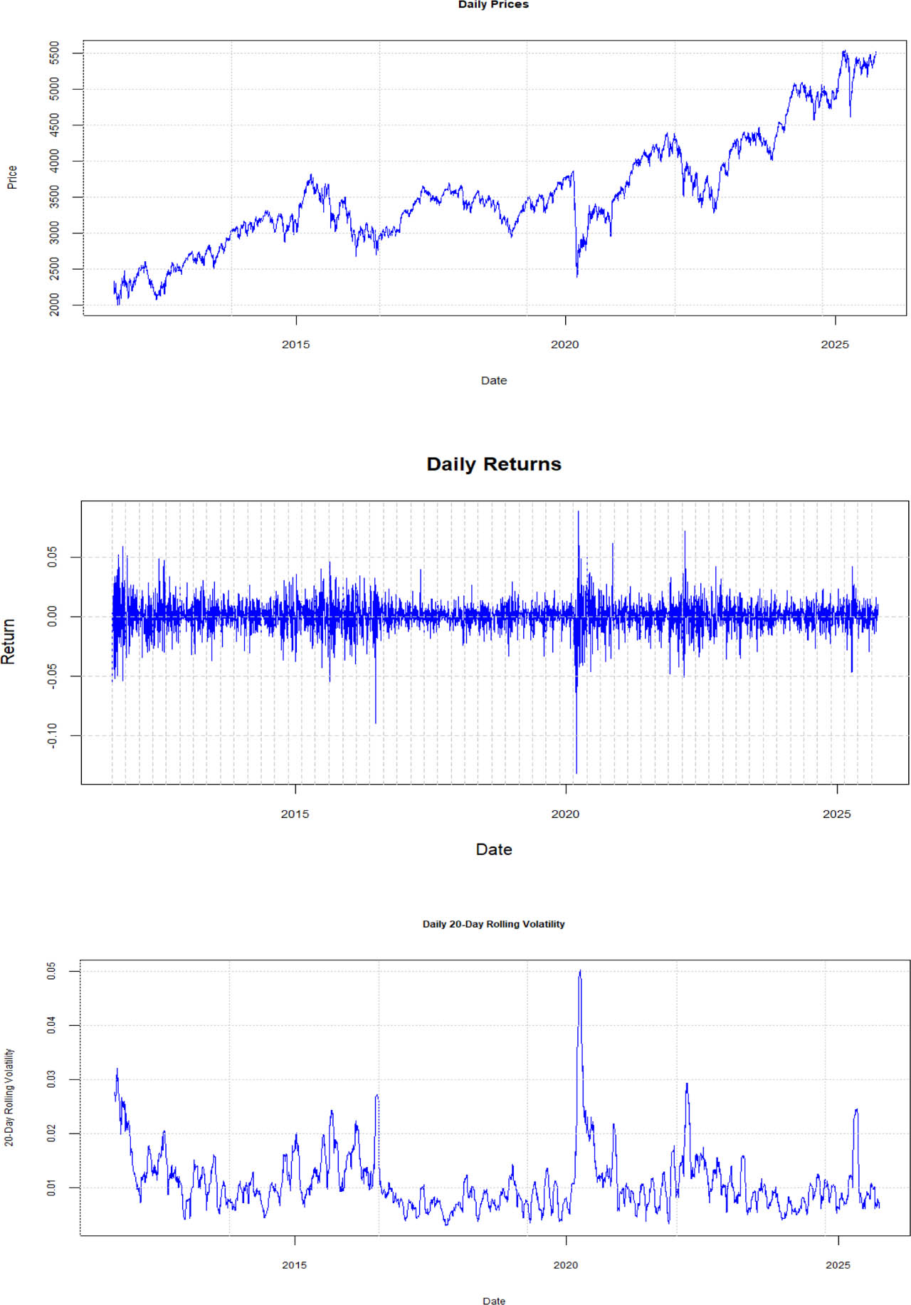
Figure 1.
Daily price, return and volatility of the Euro Stoxx 50
Note: The first part of the figure shows the daily price during the analysed period; the figure in the middle part shows the return of the analysed period; the third part shows the 20-day rolling volatility of the Euro Stoxx 50. The 20-day rolling volatility has been selected as it approximates one trading month
Figure 1 presents the patterns of daily prices, daily returns and 20-day rolling volatility of the Euro Stoxx 50 from 15 August 2011 to 30 September 2026. The daily price series demonstrates noticeable upward and downward movements over time, while the daily returns fluctuate around zero. The 20-day rolling volatility shows several spikes, indicating periods of heightened market uncertainty.
4. Methodology
In order to forecast the volatility of the selected index, GARH-type models were employed. They are as follows: GARCH(1,1), EGARCH(1,1) and GJR-GARCH(1,1). The selected models were estimated with orders (p,q)=(1,1).
The GARCH(1,1) model is widely used due to its simplicity and effectiveness in capturing volatility clustering, a common feature of financial time series in which high-volatility events tend to cluster (Naik & Reddy, 2021; Viljoen et al., 2022). It has been selected for analysis of Euro Stoxx 50 volatility, as studies have shown that GARCH models provide robust volatility estimates and are well-suited for high-frequency data, such as stock returns (Feng & Shi, 2017). Hence, using the GARCH(1,1) model for forecasting the volatility of the Euro Stoxx 50 has several advantages, including the simplicity and robustness of GARCH(1,1). The general equation of the GARCH(1,1) model can be written as follows (Aliu & Nuhiu, 2025):
where: rt - returns during period t; μ- average returns; ɛt - residual returns; α0, α1 and β1 - estimated coefficients; - conditional variance of the series; - ARCH term; - GARCH term.Another model was EGARCH(1,1). The EGARCH(1,1) model can capture asymmetry, indicating that positive and negative shocks of equal magnitude have differing influences on the conditional volatility, as well as the leverage effect (Chang & McAleer, 2017), which is one of the most powerful advantages of the model and its suitability for forecasting the volatility of the Euro Stoxx 50 index. The EGARCH(1,1) model can take the following form (Aliu & Nuhiu, 2025):
where: γ- parameter that captures the asymmetric (leverage) effect.In addition to GARCH(1,1) and EGARCH(1,1), GJR-GARCH(1,1) has been employed. Studies have demonstrated that the GJR-GARCH(1,1) model provides better out-of-sample forecasts compared to other models (Mohd Nor & Shamiri, 2007). The model's general performance in capturing asymmetric volatility and improving forecasting accuracy has been demonstrated across various financial markets (Liu & Hung, 2010; Biktimirov & Wang, 2017), making it an appropriate choice for modelling indices such as the Euro Stoxx 50. The GJR-GARCH(1,1) can be expressed in the following form (Aliu & Nuhiu, 2025):
where: It−1 - the dummy variable.To sum up, all the selected models complement each other, making them suitable choices for comprehensive volatility forecasting.
The GARCH-type models were estimated using maximum likelihood implemented in the R version 4.5.1. (R Core Team, Vienna, Austria) Estimation was carried out using the rugarch package.
5. Results and Interpretation
In order to accurately predict the volatility of the Euro Stoxx 50 (STOXX50E), three GARCH-type models were employed. They are as follows: GARCH, EGARCH and GJR-GARCH. The in-sample and out-of-sample performance metrics are presented in Tables 2 and 3.
Table 2.
In-sample parameter estimates
| Parameter | Estimate | Std. error | t-value |
|---|---|---|---|
| GARCH | |||
| μ | 0.000214 | 0.000167 | 1.2773 |
| ω | 0.000007*** | 0.000001 | 6.0969 |
| α1 | 0.064832*** | 0.002266 | 28.6155 |
| β1 | 0.934159*** | 0.006376 | 146.5103 |
| Shape | 2.593921 | 0.078449 | 33.0650 |
| AIC | −5.8302 | ||
| BIC | −5.8217 | ||
| EGARCH μ | |||
| 0.000132 | 0.000155 | 0.85105 | |
| ω | −0.174654*** | 0.003201 | −54.55830 |
| α1 | −0.153043*** | 0.015497 | −9.87557 |
| β1 | 0.979142*** | 0.000124 | 7874.31135 |
| γ1 | 0.108245*** | 0.012534 | 8.63620 |
| Shape | 2.741881 | 0.137481 | 19.94372 |
| AIC | −5.8744 | ||
| BIC | −5.8641 | ||
| GJR-GARCH μ | |||
| 0.000192 | 0.000159 | 1.207957 | |
| ω | 0.000007*** | 0.000000 | 19.769616 |
| α1 | 0.000000 | 0.004249 | 0.000003 |
| β1 | 0.923050*** | 0.007547 | 122.309813 |
| γ1 | 0.151898*** | 0.022638 | 6.709946 |
| Shape | 2.678598 | 0.093473 | 28.656460 |
| AIC | −5.8622 | ||
| BIC | −5.8519 |
[i] Note: *, ** and *** represent significance levels of 5%, 1% and 0.1%, respectively. The results show strong volatility persistence across all models and significant asymmetry in the EGARCH and GJR-GARCH models, confirming the presence of leverage effects. Based on AIC and BIC, EGARCH provides the best in-sample fit among the analysed models.
Table 3.
Out-of-sample accuracy metrics
| Model | QLIKE | MSE | MAE | HMSE | HMAE |
|---|---|---|---|---|---|
| GARCH | −7.260182 | 2.10395e-06 | 0.0004357386 | 0.004309232 | 0.02136632 |
| EGARCH | −7.352322 | 2.07787e-06 | 0.000400113 | 0.003523288 | 0.02027521 |
| GJR-GARCH | −7.32378 | 2.209141e-06 | 0.0004335917 | 0.003646335 | 0.02082398 |
[i] Note: EGARCH(1,1) outperforms both GARCH(1,1) and GJR-GARCH(1,1) in most forecast accuracy measures, particularly QLIKE, MSE and MAE, indicating the best quality volatility forecasting performance. While GJR-GARCH(1,1) performs competitively in terms of HMSE and HMAE, it does not consistently outperform EGARCH across all criteria. Overall, EGARCH provides the most stable and accurate performance among the three models.
The results of the post-estimation diagnostic tests are provided in Table 4.
Table 4.
Post-estimation diagnostic tests
| Model | LB residuals | LB squared residuals | ARCH-LM | Sign bias |
|---|---|---|---|---|
| GARCH(1,1) | 0.1227 | 0.7718 | 0.8559 | 0.0296 |
| EGARCH(1,1) | 0.1199 | 0.2361 | 0.6006 | 0.3663 |
| GJR-GARCH(1,1) | 0.1932 | 0.2286 | 0.5433 | 0.2072 |
[i] Note: The p-values from post-estimation diagnostic tests are provided in the table for all the employed models. The Ljung–Box tests applied to standardised residuals and squared standardised residuals indicate no significant serial correlation or residual ARCH effects across all specifications, as all p-values exceed 0.05. Similarly, the ARCH-LM test confirms that each model adequately captures conditional heteroskedasticity. The sign-bias test reveals evidence of asymmetric effects only in the GARCH(1,1) specification (p < 0.05), suggesting that the symmetric GARCH model does not fully capture leverage effects. Both EGARCH(1,1) and GJR-GARCH(1,1) show no significant sign bias, indicating that these asymmetric specifications adequately account for volatility asymmetry in the data. Overall, the diagnostic results support the adequacy of the EGARCH(1,1) and GJR-GARCH(1,1) models over the standard GARCH(1,1) model in capturing the underlying volatility dynamics.
The results showed that, in the GARCH(1,1) model, both α1 and β1 parameters are statistically significant, indicating that current volatility is strongly influenced by past shocks and past volatility. Moreover, the sum of these parameters is close to 1, indicating that volatility is highly persistent and that shocks have a long-lasting effect. The μ parameter is statistically significant, representing the mean return of the series, that is, the average daily return of the Euro Stoxx 50 Index is slightly positive. The ω parameter is also significant, albeit very small, indicating that it is driven by recent shocks and past volatility rather than a constant baseline component. In the EGARCH(1,1) model, all parameters are statistically significant, except μ. The negative, statistically significant coefficient of α1 indicates a clear asymmetric volatility pattern. The value of β1 is close to 1, indicating that past volatility has a strong influence on current volatility. Moreover, in the EGARCH(1,1) model, the leverage parameter γ1 is also significant, indicating asymmetry: negative shocks have a different effect on volatility than positive shocks of the same magnitude. In fact, the leverage effect implies that negative shocks tend to increase volatility more than positive shocks (Chen & Gankhuyag, 2022). The ω parameter is negative and significant, indicating that the baseline volatility is low; therefore, in the absence of shocks, the model starts at a low volatility level. The insignificant α1 coefficient in the GJR-GARCH (1,1) model suggests that symmetric shock effects are weak, while volatility dynamics are mainly explained by the persistence term and the significant asymmetric effect of negative shocks. Moreover, in the model, the coefficient of γ1 is positive and statistically significant, indicating that negative shocks increase volatility more than positive shocks of the same magnitude, thereby confirming the presence of the leverage effect. The high, significant β1 indicates strong volatility persistence. The ω parameter is statistically significant but very small (similar to the GARCH model), indicating that a minimal baseline level of volatility in the Euro Stoxx 50 Index persists even in the absence of new shocks.
It should be noted that both the Akaike information criterion (AIC) and the Bayesian information criterion (BIC) are lowest for the EGARCH model, indicating that this specification provides the best in-sample fit. The out-of-sample performance assessment is based on QLIKE, MSE, MAE, HMSE and HMAE metrics. These measures assess the accuracy of volatility forecasts, where lower values indicate better performance. Among the three models, EGARCH achieves the lowest values across all criteria, demonstrating superior forecasting performance compared to the other two.
Overall, comparisons among GARCH-type models for forecasting volatility in the Index in the Eurozone are rare; thus, it is difficult to accurately compare the results in this article with those of other authors. But other authors also noted that the EGARCH model consistently outperforms alternatives (Sanz-Martín et al., 2025b; Vasiljeva, Matvejevs & Fjodorovs, 2025), while others confirmed that models that use realised volatility (RV) (RSV, REGARCH) outperform those that do not (EGARCH), suggesting that RV provides useful information in forecasting volatility (Takahashi, Watanabe & Omori, 2024). Some authors (Malik, Ewing & Payne, 2005; Kang, Cho & Yoon, 2009; Fatima, Gan & Hu, 2022) used them for volatility analysis of precious metals in the Eurozone, and the results were similar to existing ones—when the simple GARCH model is used without correction, there is a significant negative relationship between the respective market share price index and the gold, silver and platinum markets. Naimy et al. (2023) employed GARCH-type models to examine post-Brexit exchange rate volatility and its effects on UK exports to the Eurozone. The results showed that the GARCH(1,1) model best captured exchange rate volatility before and after the Brexit vote. Still, when the authors introduced a dummy variable to test whether the exchange rate's volatility structure changed after the Brexit vote, the results did not provide significant evidence.
Volatility in the Eurozone is a dynamic concept, and ongoing research is necessary to capture the full range of factors that affect it. MacDonald, Sogiakas and Tsopanakis (2018) employed a multivariate GARCH approach, utilising financial stress indices as systemic risk metrics. They identified that the main recipients and transmitters of spillover effects vary across sectors. As per MacDonald et al. (2018), interconnected European markets exhibit clear disaggregation when adverse economic events occur in peripheral economies, leading to markets interacting and becoming susceptible to the effects of their respective country groups. Investors tend to flee debt-ridden economies, seeking safer, more stable investment opportunities in less volatile markets.
The GARCH-type models are beneficial for their ability to reproduce a wide range of volatility dynamics and model time-varying, asymmetric volatility; thus, as observed in this scientific paper, the Euro Stoxx 50 index reacts differently to positive and negative shocks. However, further research is needed to confirm these findings and identify factors that influence volatility in the Eurozone. Studies such as those by Fatima et al. (2022), Kang et al. (2009), and Malik et al. (2005) show that simple GARCH models often reveal a significant negative relationship between Eurozone stock indices and precious metals (gold, silver and platinum). However, when dummy variables are introduced, this relationship weakens or disappears, suggesting that structural breaks or regime changes can significantly alter volatility dynamics. The inclusion of dummy variables in GARCH models appears to correct or reduce volatility persistence, as noted by Fatima et al. (2022). This implies that accounting for specific events or periods (e.g., crises, policy changes) can improve model accuracy and realism.
The current scientific paper confirms that the Euro Stoxx 50 index exhibits mild asymmetry in its response to shocks—negative shocks tend to have a stronger impact on volatility than positive ones. This behaviour is well captured by models like EGARCH, which are designed to handle asymmetric effects. There may be several economic and geopolitical factors that explain the observed results. Nowadays, geopolitical risk is rising, including tensions in the Middle East, United States-China relations, the Russia–Ukraine conflict and the Hamas–Israel conflict in 2023; thus, European markets react more sharply to negative geopolitical shocks than to positive developments. Sudden changes in trade or defence policies, including United States tariffs and European Union defence spending, disproportionately affect investor sentiment, leading to sharper volatility increases during negative news cycles.
The Euro Stoxx 50 index also reacts with stronger, more persistent behavioural responses to negative news. Typically, loss aversion manifests as investors reacting more strongly to negative news than to positive news, and this behavioural bias leads to larger volatility spikes following negative returns, which explains the significant negative α1 and positive γ1 in EGARCH and GJR-GARCH models. The Eurozone experienced slow GDP growth of 1.1% in Q3 2025, and inflation remains above the European Central Bank's target of 3.71% in 2025, contributing to prolonged uncertainty and persistent volatility in financial markets.
6. Conclusions
Volatility in the Eurozone is a dynamic concept, as turbulent events in global markets have driven capital toward alternative and relatively safer investment opportunities in more stable markets. The Euro Stoxx 50 Index has recently attracted attention from advanced econometric frameworks, creating opportunities for volatility management. The need for more active research in volatility management is obvious. The present results revealed that the volatility of the Euro Stoxx 50 index is persistent and mildly asymmetric, that is, the reactions to positive and negative shocks differ slightly. The empirical estimation of GARCH-type models for the Euro Stoxx 50(STOXX50) reveals distinct volatility dynamics and clear structural differences in model performance. All this information is better captured by the EGARCH model, which not only provides the best in-sample fit according to AIC and BIC but also generates the most accurate out-of-sample volatility prediction. Modern research on GARCH-type models in financial forecasting indicates that asymmetric performance remains foundational for volatility forecasting. GARCH-type models are beneficial because they can reproduce a wide range of volatility dynamics and model time-varying, asymmetric volatility. The EGARCH model captures both volatility clustering and asymmetry compared to other models in the present research, making it particularly well-suited for the Euro Stoxx 50, which is sensitive to frequent geopolitical shocks, such as trade wars, military conflicts and economic policy uncertainty, including European Central Bank rate decisions, inflation control and others.
GARCH-type models are showing consistent volatility forecasts for the Euro Stoxx 50 in the Eurozone; models that integrate the latest neural networks are also competing to better capture volatility. This limits the ability to benchmark the current findings against a broad body of existing research, highlighting a gap in the literature and an opportunity for further empirical studies in this region. To finalise, Eurozone market volatility remains a highly dynamic, asymmetric phenomenon deeply rooted in regional and global systemic risk networks. Given the dynamic nature of volatility in the Eurozone and the influence of macroeconomic, geopolitical and sectoral factors, ongoing research is essential. Future studies should explore more complex models, incorporate additional explanatory variables and consider structural breaks to better understand and forecast volatility more accurately. Moreover, some Eurozone economies still face fragile fiscal positions post-COVID, and rising defence spending adds to long-term instability in financial markets, given the interconnectedness of European markets.