

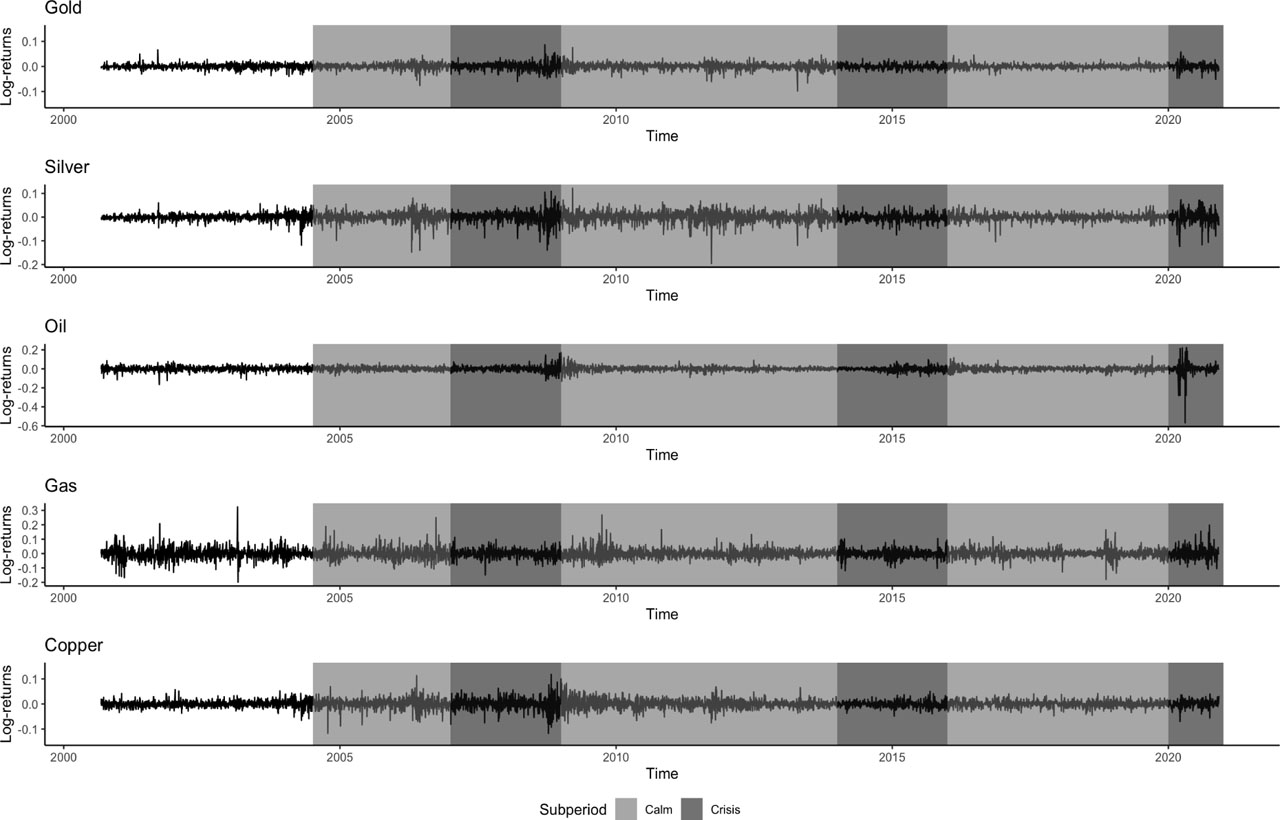
Figure 1.
Returns for commodities (light grey for calm period, dark grey for crisis period)
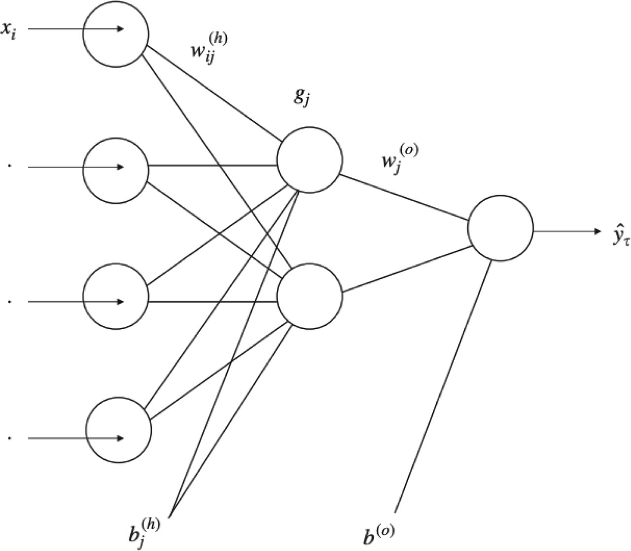
Figure 2.
The diagram of QRNN model with four predictors and two hidden nodes Source: Cannon, 2011
Table 1.
Statistics of prices’ log-returns
| Commodity | Min. | 1st Qu. | Median | Mean | 3rd Qu. | Max | J-B test | Skewness | Ex. Kurtosis |
|---|---|---|---|---|---|---|---|---|---|
| Gold | −0.0982 | −0.0049 | 0.0005 | 0.0004 | 0.006 | 0.0864 | 6398 (<0.001) | –0.2658 | 8.7160 |
| Silver | −0.1955 | −0.0080 | 0.0011 | 0.0003 | 0.0090 | 0.1220 | 13942 (<0.001) | –0.9263 | 10.8079 |
| Oil | −0.2799 | −0.0128 | 0.0008 | 0.0001 | 0.0130 | 0.3196 | 52559 (<0.001) | –1.9164 | 52.6291 |
| Gas | −0.1990 | −0.1911 | −0.0007 | −0.0001 | 0.0173 | 0.3238 | 6833 (<0.001) | 0.5643 | 8.7537 |
| Copper | −0.1169 | −0.0082 | 0.0002 | 0.0003 | 0.0089 | 0.1177 | 4279 (<0.001) | –0.1731 | 7.6239 |
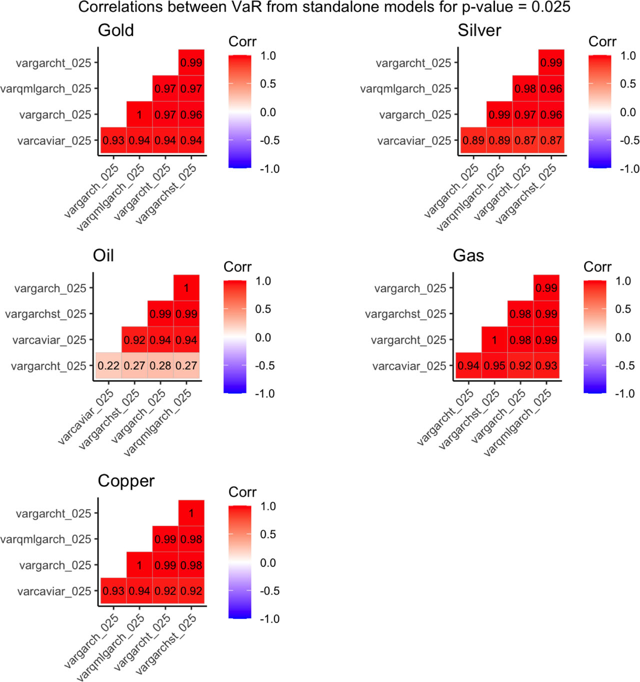
Figure 3.
Correlations between VaR forecasts for p-value = 0.025
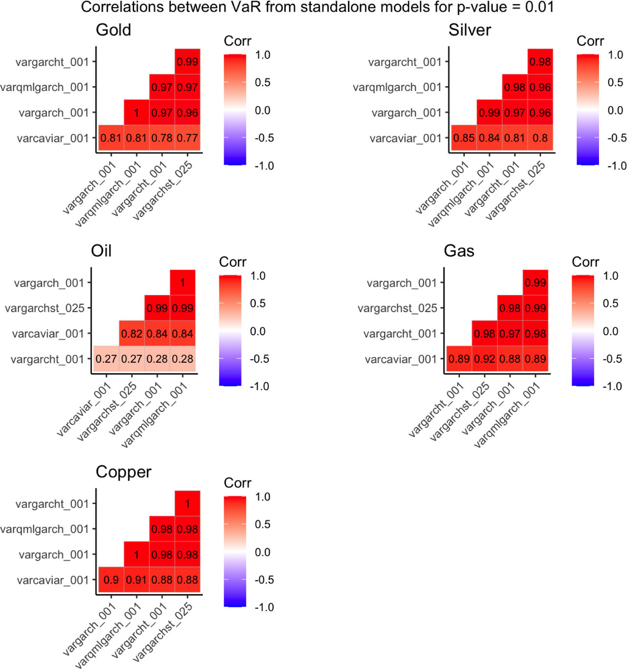
Figure 4.
Correlations between VaR forecasts for p-value = 0.01
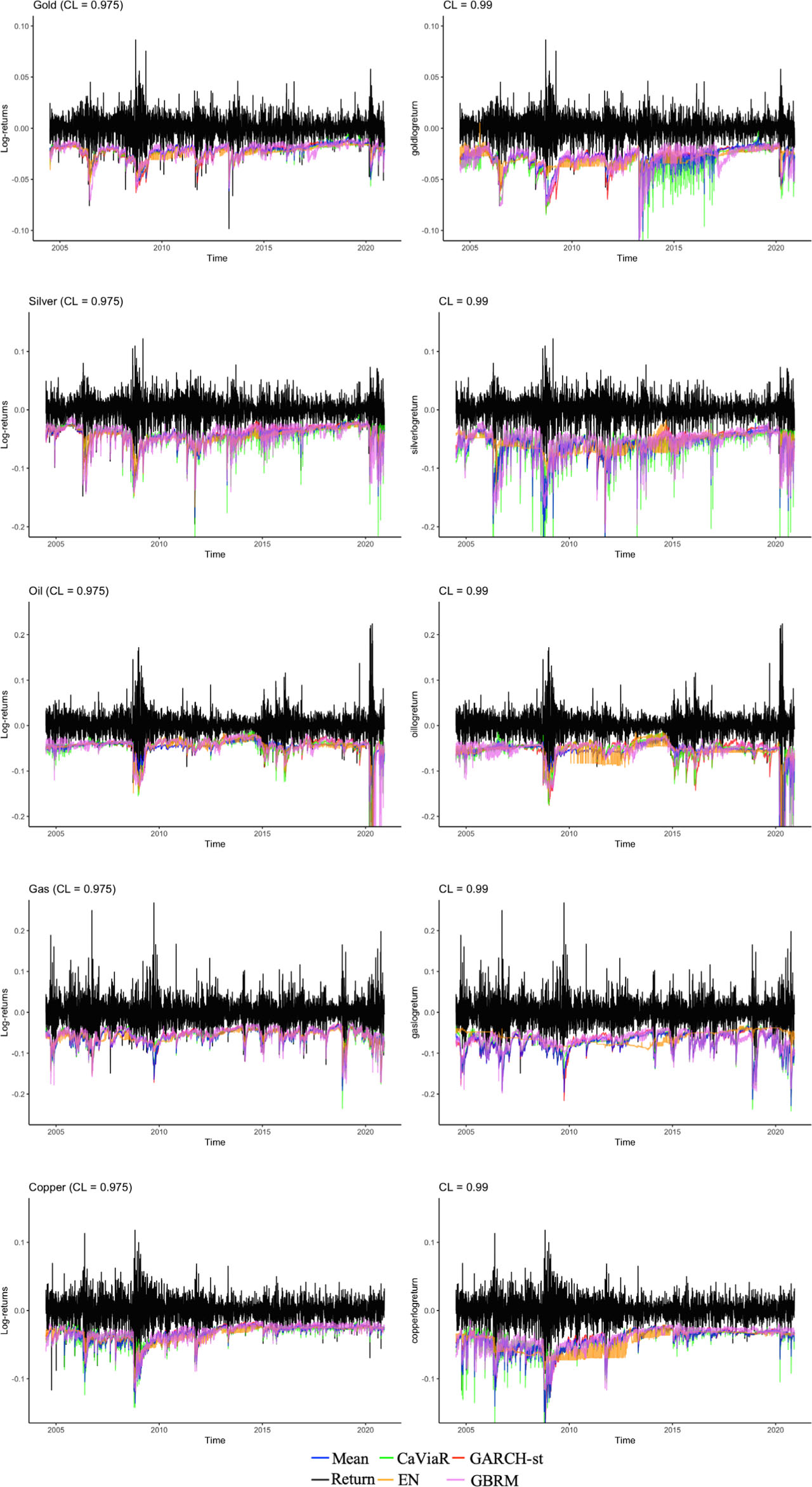
Figure 5.
Returns and VaR forecast for confidence levels: 0.975 (on left) and 0.99 (on right)
Table 2.
Test results: Excess Ratio (ER), Kupiec (UC), Christoffersen (CC), Dynamic Quantile (DQ) and Traffic Light (TL) divided into the analysed models and periods for gold for confidence level equal to 0.975
| Model | Period I (Whole period) | Period II (All calm periods) | Period I (All crisis periods) | Period I (COVID period) | ||||||||||||||||
|---|---|---|---|---|---|---|---|---|---|---|---|---|---|---|---|---|---|---|---|---|
| ER | UC | CC | DQ | TL | ER | UC | CC | DQ | TL | ER | UC | CC | DQ | TL | ER | UC | CC | DQ | TL | |
| GARCH | 3.10% | 5.77 | 6.02 | 21.07 | Y | 2.85% | 1.38 | 1.55 | 9.22 | G | 3.70% | 6.45 | 6.50 | 16.92 | Y | 5.63% | 6.88 | 6.98 | 26.48 | Y |
| GARCH-t | 2.81% | 1.62 | 1.77 | 18.08 | G | 2.57% | 0.06 | 0.07 | 2.48 | G | 3.38% | 3.57 | 3.80 | 28.92 | Y | 4.76% | 3.85 | 4.23 | 21.16 | Y |
| GARCH-st | 2.38% | 0.24 | 0.41 | 16.80 | G | 2.20% | 1.16 | 1.29 | 5.88 | G | 2.82% | 0.50 | 1.36 | 21.53 | G | 4.33% | 2.61 | 3.22 | 22.78 | Y |
| QML-GARCH | 3.17% | 5.91 | 6.02 | 22.59 | Y | 2.88% | 1.66 | 1.80 | 9.14 | G | 3.62% | 5.66 | 5.74 | 19.26 | Y | 5.59% | 6.80 | 6.98 | 26.36 | Y |
| CaViaR | 2.65% | 0.36 | 0.74 | 20.85 | G | 2.47% | 0.01 | 0.04 | 15.69 | G | 3.06% | 1.49 | 2.02 | 14.36 | G | 5.19% | 5.28 | 7.53 | 31.81 | Y |
| Mean | 2.81% | 1.62 | 1.77 | 14.83 | G | 2.64% | 0.24 | 0.24 | 9.74 | G | 3.22% | 2.43 | 2.79 | 11.04 | Y | 4.76% | 3.85 | 4.23 | 15.45 | Y |
| Highest VaR | 3.46% | 14.18 | 14.38 | 41.56 | R | 3.19% | 5.25 | 5.25 | 15.70 | Y | 4.11% | 11.05 | 11.42 | 33.81 | Y | 6.49% | 10.57 | 11.54 | 41.72 | Y |
| Lowest VaR | 2.07% | 3.37 | 3.39 | 10.49 | G | 1.92% | 4.35 | 4.36 | 8.59 | G | 2.42% | 0.04 | 0.14 | 7.87 | G | 3.46% | 0.79 | 2.04 | 7.83 | G |
| CQOM | 2.69% | 0.63 | 9.01 | 56.89 | G | 2.47% | 0.01 | 4.21 | 39.29 | G | 3.25% | 2.48 | 6.46 | 44.63 | Y | 3.90% | 1.58 | 2.48 | 11.99 | G |
| Elastic Net | 2.50% | 0.00 | 1.85 | 24.77 | G | 2.20% | 1.16 | 1.39 | 7.99 | G | 3.27% | 2.49 | 4.23 | 30.53 | Y | 6.49% | 10.57 | 11.54 | 81.74 | Y |
| LASSO | 2.62% | 0.25 | 6.95 | 30.04 | G | 2.26% | 0.69 | 6.14 | 14.90 | G | 3.46% | 4.22 | 5.51 | 44.51 | Y | 7.36% | 14.83 | 15.27 | 91.46 | R |
| QRF | 5.15% | 92.01 | 92.12 | 246.98 | R | 4.87% | 52.90 | 52.90 | 158.42 | R | 5.80% | 40.61 | 41.02 | 93.76 | R | 8.66% | 22.16 | 22.59 | 57.90 | R |
| GBRM | 2.89% | 2.43 | 2.51 | 16.97 | G | 2.57% | 0.06 | 0.07 | 5.19 | G | 3.62% | 5.66 | 5.74 | 19.85 | Y | 4.76% | 3.85 | 4.23 | 17.65 | Y |
| QRNN | 4.71% | 66.66 | 70.04 | 223.39 | R | 4.49% | 38.60 | 39.35 | 105.05 | R | 5.23% | 29.10 | 32.44 | 212.53 | R | 9.09% | 24.82 | 29.35 | 176.38 | R |
[i] Note: Gray fields indicate p-values greater than 5%. GARCH stands for GARCH(1,1), GARCH-t - AR-GARCH-t(1,1), GARCH-st - AR-GARCH(1,1), QML-GARCH - QML-GARCH(1,1), CaViaR - Indirect GARCH(1,1), Mean stands for simple average from GARCH and CaViaR, Highest VaR means the maximum from GARCH, GARCH-t, GARCH-st, QML-GARCH, and CaViaR, Lowest VaR stands for the minimum from individual models, CQOM stands for Conditional Quantile Optimisation Method applied for GARCH and CaViaR (described in section 2.3.4), Elastic Net stands for forecast combined using quantile regression with elastic net regularisation (described in section 2.3.6), LASSO stands for forecast combined using quantile regression with LASSO regularisation (described in section 2.3.5), QRF stands for forecast combined using Quantile Regression Forests (described in section 2.3.7), GBRM stands for forecast combined using Gradient Boosting Regression Model (described in section 2.3.8), QRNN stands for forecast combined using Quantile Regression Neural Network (described in section 2.3.9). In TL: 1) G stands for green, 2) Y stands for yellow, 3) R stands for red.
Table 3.
Test results: Excess Ratio (ER), Kupiec (UC), Christoffersen (CC), Dynamic Quantile (DQ) and Traffic Light (TL) divided into the analysed models and periods for gold for confidence level equal to 0.99
| Model | Period I (Whole period) | Period II (All calm periods) | Period I (All crisis periods) | Period I (COVID period) | ||||||||||||||||
|---|---|---|---|---|---|---|---|---|---|---|---|---|---|---|---|---|---|---|---|---|
| ER | UC | CC | DQ | TL | ER | UC | CC | DQ | TL | ER | UC | CC | DQ | TL | ER | UC | CC | DQ | TL | |
| GARCH | 1.85% | 24.38 | 24.59 | 47.78 | R | 1.65% | 10.30 | 10.36 | 20.23 | Y | 2.33% | 16.25 | 16.39 | 40.37 | R | 3.46% | 8.64 | 9.89 | 31.80 | Y |
| GARCH-t | 1.13% | 0.69 | 6.40 | 18.19 | G | 1.06% | 0.12 | 1.02 | 3.17 | G | 1.29% | 0.96 | 6.88 | 34.25 | G | 2.19% | 2.39 | 5.38 | 30.03 | Y |
| GARCH-st | 0.91% | 0.32 | 4.16 | 9.17 | G | 0.89% | 0.36 | 1.79 | 3.81 | G | 0.97% | 0.01 | 2.69 | 9.69 | G | 2.16% | 2.37 | 5.38 | 30.07 | Y |
| QML-GARCH | 1.90% | 24.66 | 24.59 | 47.38 | R | 1.67% | 10.35 | 10.36 | 20.02 | Y | 2.37% | 16.43 | 16.39 | 40.04 | R | 3.55% | 8.87 | 9.89 | 31.55 | Y |
| CaViaR | 1.03% | 0.05 | 3.07 | 15.54 | G | 1.10% | 0.27 | 1.09 | 6.80 | G | 0.89% | 0.17 | 3.18 | 13.09 | G | 2.60% | 4.13 | 6.42 | 26.36 | Y |
| Mean | 1.30% | 3.43 | 5.09 | 18.31 | Y | 1.30% | 2.48 | 2.89 | 8.34 | G | 1.29% | 0.96 | 2.61 | 18.09 | G | 3.46% | 8.64 | 9.89 | 31.23 | Y |
| Highest VaR | 1.88% | 25.64 | 26.93 | 52.17 | R | 1.65% | 10.30 | 10.36 | 19.95 | Y | 2.42% | 18.01 | 19.63 | 49.68 | R | 3.46% | 8.64 | 9.89 | 31.27 | Y |
| Lowest VaR | 0.84% | 1.11 | 5.53 | 12.07 | G | 0.86% | 0.63 | 2.19 | 3.78 | G | 0.81% | 0.51 | 3.89 | 13.52 | G | 2.16% | 2.37 | 5.38 | 30.17 | Y |
| CQOM | 1.54% | 10.50 | 13.28 | 51.94 | Y | 1.44% | 5.04 | 7.12 | 34.06 | Y | 1.77% | 6.07 | 6.77 | 35.15 | Y | 2.60% | 4.13 | 6.42 | 52.00 | Y |
| Elastic Net | 1.32% | 3.98 | 11.47 | 62.74 | Y | 1.10% | 0.27 | 8.30 | 39.08 | G | 1.85% | 7.28 | 7.86 | 40.96 | Y | 3.46% | 8.64 | 9.89 | 43.82 | Y |
| LASSO | 1.27% | 2.92 | 4.68 | 34.99 | Y | 1.06% | 0.12 | 1.02 | 7.58 | G | 1.77% | 6.07 | 6.77 | 42.25 | Y | 3.90% | 11.30 | 12.19 | 48.62 | Y |
| QRF | 3.61% | 171.00 | 171.03 | 448.16 | R | 3.64% | 122.05 | 122.39 | 323.10 | R | 3.54% | 48.97 | 52.20 | 148.36 | R | 4.76% | 17.29 | 18.39 | 73.79 | R |
| GBRM | 1.35% | 4.56 | 11.81 | 80.37 | Y | 0.96% | 0.05 | 4.83 | 17.66 | G | 2.25% | 14.56 | 16.57 | 99.99 | R | 2.60% | 4.13 | 6.42 | 47.14 | Y |
| QRNN | 3.42% | 150.49 | 160.82 | 541.10 | R | 3.29% | 96.70 | 102.40 | 349.83 | R | 3.70% | 54.22 | 58.90 | 206.00 | R | 6.06% | 27.68 | 27.71 | 80.57 | R |
[i] Note: The same as for the pervious table.
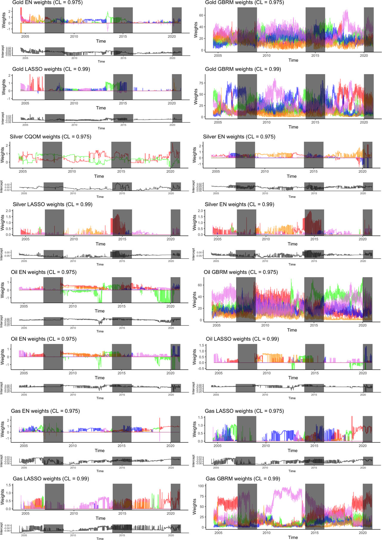
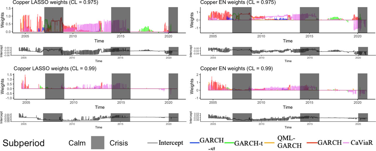
Figure 6.
Combing weight for the most promising methods of combining VaR forecasts for all assets for both confidence levels (CL)—0.975 and 0.99
Table 4.
Test results: Excess Ratio (ER), Kupiec (UC), Christoffersen (CC), Dynamic Quantile (DQ) and Traffic Light (TL) divided into the analysed models and periods for silver for confidence level equal to 0.975.
| Model | Period I (Whole period) | Period II (All calm periods) | Period I (All crisis periods) | Period I (COVID period) | ||||||||||||||||
|---|---|---|---|---|---|---|---|---|---|---|---|---|---|---|---|---|---|---|---|---|
| ER | UC | CC | DQ | TL | ER | UC | CC | DQ | TL | ER | UC | CC | DQ | TL | ER | UC | CC | DQ | TL | |
| GARCH | 3.58% | 17.72 | 21.25 | 41.94 | R | 3.46% | 9.96 | 11.56 | 22.90 | Y | 3.86% | 8.16 | 10.22 | 22.05 | Y | 5.63% | 3.85 | 6.69 | 28.62 | Y |
| GARCH-t | 3.42% | 12.86 | 21.07 | 38.19 | Y | 3.16% | 4.76 | 9.27 | 19.21 | Y | 4.03% | 10.04 | 13.55 | 24.26 | Y | 4.76% | 2.85 | 6.14 | 22.35 | Y |
| GARCH-st | 2.91% | 2.74 | 13.82 | 34.46 | Y | 2.68% | 0.36 | 8.13 | 24.97 | G | 3.46% | 4.22 | 7.42 | 16.69 | Y | 4.33% | 2.74 | 6.14 | 23.15 | Y |
| QML-GARCH | 3.44% | 13.51 | 21.50 | 43.07 | R | 3.40% | 8.65 | 11.93 | 24.52 | Y | 3.54% | 4.91 | 10.27 | 22.85 | Y | 5.69% | 2.90 | 6.14 | 23.09 | Y |
| CaViaR | 2.84% | 1.87 | 3.74 | 25.47 | G | 2.64% | 0.24 | 0.24 | 9.71 | G | 3.30% | 2.98 | 6.86 | 29.91 | Y | 5.19% | 10.57 | 11.72 | 38.85 | Y |
| Mean | 2.77% | 1.17 | 4.91 | 16.11 | G | 2.47% | 0.01 | 0.75 | 5.15 | G | 3.46% | 4.22 | 7.55 | 18.32 | Y | 4.76% | 6.88 | 8.88 | 31.12 | Y |
| Highest VaR | 4.14% | 38.32 | 44.18 | 74.44 | R | 3.81% | 17.68 | 20.61 | 38.17 | R | 4.91% | 23.23 | 25.99 | 42.50 | R | 6.49% | 12.63 | 13.45 | 34.59 | R |
| Lowest VaR | 2.21% | 1.46 | 6.86 | 19.48 | G | 2.09% | 2.10 | 2.47 | 10.64 | G | 2.50% | 0.00 | 7.41 | 22.49 | G | 3.46% | 2.61 | 6.14 | 30.82 | Y |
| CQOM | 2.38% | 0.24 | 18.45 | 51.46 | G | 2.16% | 1.44 | 14.15 | 34.88 | G | 2.90% | 0.77 | 6.12 | 20.39 | G | 3.90% | 2.69 | 6.14 | 27.15 | Y |
| Elastic Net | 2.48% | 0.01 | 8.00 | 30.60 | G | 2.30% | 0.50 | 3.40 | 15.17 | G | 2.91% | 0.78 | 6.12 | 22.45 | G | 6.49% | 3.85 | 6.69 | 34.39 | Y |
| LASSO | 2.72% | 0.79 | 17.15 | 72.79 | G | 2.26% | 0.69 | 12.27 | 39.12 | G | 3.78% | 7.28 | 11.65 | 55.77 | Y | 7.36% | 17.15 | 17.42 | 73.08 | R |
| QRF | 4.81% | 72.00 | 73.95 | 217.41 | R | 4.39% | 35.03 | 35.37 | 107.96 | R | 5.80% | 40.61 | 42.44 | 126.89 | R | 8.66% | 10.57 | 10.57 | 55.56 | Y |
| GBRM | 3.32% | 10.41 | 19.53 | 59.65 | Y | 3.05% | 3.42 | 6.62 | 22.87 | Y | 3.95% | 9.08 | 15.27 | 47.33 | Y | 4.76% | 6.88 | 8.63 | 29.33 | Y |
| QRNN | 5.00% | 83.19 | 102.20 | 395.17 | R | 4.70% | 46.17 | 55.58 | 253.17 | R | 5.72% | 38.88 | 48.45 | 157.84 | R | 9.09% | 39.66 | 40.11 | 147.69 | R |
[i] Note: The same as for the table 2, but here GARCH stands for GARCH(1,2), QML-GARCH stands for AR-QML-GARCH(1,1), Mean stands for simple average from GARCH-st and CaViaR.
Table 5.
Test results: Excess Ratio (ER), Kupiec (UC), Christoffersen (CC), Dynamic Quantile (DQ) and Traffic Light (TL) divided into the analysed models and periods for silver for confidence level equal to 0.99
| Model | Period I (Whole period) | Period II (All calm periods) | Period I (All crisis periods) | Period I (COVID period) | ||||||||||||||||
|---|---|---|---|---|---|---|---|---|---|---|---|---|---|---|---|---|---|---|---|---|
| ER | UC | CC | DQ | TL | ER | UC | CC | DQ | TL | ER | UC | CC | DQ | TL | ER | UC | CC | DQ | TL | |
| GARCH | 2.36% | 56.00 | 62.62 | 114.64 | R | 2.30% | 36.32 | 39.22 | 67.05 | R | 2.50% | 19.83 | 23.85 | 56.09 | R | 3.46% | 12.30 | 15.63 | 76.45 | Y |
| GARCH-t | 1.30% | 3.43 | 19.68 | 58.92 | Y | 1.06% | 0.12 | 8.50 | 25.70 | G | 1.85% | 7.28 | 14.45 | 46.95 | Y | 2.23% | 11.52 | 15.63 | 73.12 | Y |
| GARCH-st | 1.03% | 0.05 | 21.68 | 77.52 | G | 0.75% | 1.94 | 14.40 | 42.41 | G | 1.69% | 4.96 | 13.18 | 47.30 | Y | 2.16% | 11.30 | 15.63 | 75.03 | Y |
| QML-GARCH | 2.31% | 52.56 | 62.26 | 120.78 | R | 2.20% | 31.39 | 34.78 | 61.32 | R | 2.58% | 21.72 | 28.68 | 71.24 | R | 3.51% | 12.73 | 15.63 | 74.50 | Y |
| CaViaR | 1.11% | 0.46 | 3.05 | 19.34 | G | 0.93% | 0.16 | 1.48 | 4.38 | G | 1.53% | 3.03 | 4.14 | 39.88 | Y | 2.60% | 20.58 | 20.79 | 88.35 | R |
| Mean | 1.01% | 0.00 | 11.44 | 36.79 | G | 0.82% | 0.98 | 12.38 | 38.30 | G | 1.45% | 2.22 | 3.49 | 11.08 | Y | 3.46% | 11.90 | 12.19 | 48.59 | Y |
| Highest VaR | 2.65% | 78.37 | 84.86 | 157.60 | R | 2.44% | 43.32 | 45.64 | 76.26 | R | 3.14% | 36.67 | 41.01 | 101.95 | R | 3.46% | 31.46 | 32.44 | 130.63 | R |
| Lowest VaR | 0.70% | 4.29 | 10.09 | 20.68 | G | 0.62% | 4.99 | 7.69 | 9.93 | G | 0.89% | 0.17 | 3.18 | 21.35 | G | 2.16% | 4.13 | 6.42 | 55.81 | Y |
| CQOM | 1.64% | 14.24 | 29.29 | 108.75 | R | 1.51% | 6.61 | 19.03 | 76.54 | Y | 1.93% | 8.57 | 11.55 | 52.32 | Y | 2.60% | 11.60 | 12.19 | 54.94 | Y |
| Elastic Net | 1.30% | 3.43 | 19.68 | 87.01 | Y | 1.10% | 0.27 | 8.30 | 44.48 | G | 1.77% | 6.07 | 13.76 | 55.34 | Y | 3.46% | 14.19 | 17.72 | 82.18 | R |
| LASSO | 1.20% | 1.62 | 24.93 | 104.71 | G | 1.06% | 0.12 | 13.66 | 64.24 | G | 1.53% | 3.03 | 12.44 | 50.30 | Y | 3.90% | 11.93 | 15.63 | 65.06 | Y |
| QRF | 2.89% | 99.07 | 99.71 | 290.41 | R | 2.64% | 54.69 | 56.27 | 136.88 | R | 3.46% | 46.41 | 46.60 | 187.82 | R | 4.76% | 13.24 | 12.03 | 98.63 | Y |
| GBRM | 1.56% | 11.38 | 23.52 | 68.29 | Y | 1.41% | 4.32 | 13.57 | 42.35 | Y | 1.93% | 8.57 | 11.55 | 40.85 | Y | 2.60% | 2.37 | 11.96 | 92.74 | Y |
| QRNN | 3.61% | 171.00 | 177.55 | 776.88 | R | 3.46% | 109.12 | 115.76 | 459.11 | R | 3.95% | 62.45 | 63.00 | 339.63 | R | 6.06% | 47.94 | 48.22 | 305.35 | R |
[i] Note: The same as for the previous table.
Table 6.
Test results: Excess Ratio (ER), Kupiec (UC), Christoffersen (CC), Dynamic Quantile (DQ) and Traffic Light (TL) divided into the analysed models and periods for oil for confidence level equal to 0.975.
| Model | Period I (Whole period) | Period II (All calm periods) | Period I (All crisis periods) | Period I (COVID period) | ||||||||||||||||
|---|---|---|---|---|---|---|---|---|---|---|---|---|---|---|---|---|---|---|---|---|
| ER | UC | CC | DQ | TL | ER | UC | CC | DQ | TL | ER | UC | CC | DQ | TL | ER | UC | CC | DQ | TL | |
| GARCH | 2.96% | 3.39 | 3.43 | 10.66 | Y | 2.37% | 0.22 | 3.56 | 7.97 | G | 4.35% | 14.30 | 15.37 | 19.82 | R | 5.63% | 6.88 | 8.63 | 20.99 | Y |
| GARCH-t | 3.54% | 16.26 | 37.79 | 313.36 | R | 1.75% | 7.51 | 8.57 | 55.08 | G | 7.73% | 90.37 | 99.57 | 311.51 | R | 4.76% | 22.16 | 24.91 | 157.82 | R |
| GARCH-st | 2.43% | 0.09 | 0.95 | 5.04 | G | 1.96% | 3.83 | 6.10 | 8.43 | G | 3.54% | 4.91 | 7.86 | 9.45 | Y | 4.33% | 2.61 | 6.14 | 21.69 | Y |
| QML-GARCH | 3.04% | 3.53 | 3.43 | 10.71 | Y | 2.39% | 0.24 | 3.56 | 8.09 | G | 4.35% | 14.30 | 15.37 | 19.84 | R | 5.77% | 6.97 | 8.63 | 20.99 | Y |
| CaViaR | 2.57% | 0.09 | 1.66 | 14.89 | G | 1.96% | 3.83 | 3.84 | 7.94 | G | 4.03% | 10.04 | 11.73 | 24.06 | Y | 5.19% | 3.85 | 6.69 | 21.18 | Y |
| Mean | 2.50% | 0.00 | 0.68 | 18.03 | G | 1.37% | 18.14 | 19.25 | 26.72 | G | 5.15% | 27.59 | 27.74 | 37.72 | R | 4.76% | 5.28 | 5.49 | 11.16 | Y |
| Highest VaR | 4.86% | 74.74 | 83.96 | 264.82 | R | 3.16% | 4.76 | 4.76 | 29.49 | Y | 8.86% | 125.64 | 131.16 | 328.47 | R | 6.49% | 39.66 | 41.25 | 172.61 | R |
| Lowest VaR | 1.59% | 16.27 | 18.80 | 24.20 | G | 0.99% | 34.98 | 35.56 | 29.30 | G | 2.98% | 1.10 | 3.52 | 7.61 | G | 3.46% | 0.25 | 1.96 | 6.54 | G |
| CQOM | 3.01% | 4.12 | 22.26 | 157.69 | Y | 1.78% | 6.80 | 6.81 | 45.91 | G | 5.88% | 42.38 | 56.14 | 181.95 | R | 3.90% | 27.60 | 34.10 | 133.16 | R |
| Elastic Net | 2.98% | 3.75 | 5.04 | 22.36 | Y | 1.96% | 3.83 | 3.84 | 9.29 | G | 5.39% | 32.24 | 32.77 | 59.60 | R | 6.49% | 14.83 | 15.27 | 63.54 | R |
| LASSO | 3.03% | 4.51 | 10.03 | 69.61 | Y | 1.78% | 6.80 | 7.78 | 12.84 | G | 5.96% | 44.17 | 45.66 | 108.55 | R | 7.36% | 17.15 | 18.83 | 85.82 | R |
| QRF | 5.82% | 137.72 | 139.48 | 253.06 | R | 5.28% | 70.54 | 70.63 | 217.80 | R | 7.09% | 72.17 | 74.44 | 124.92 | R | 8.66% | 19.60 | 25.83 | 74.65 | R |
| GBRM | 3.39% | 12.23 | 12.24 | 24.87 | Y | 2.81% | 1.13 | 2.11 | 15.93 | G | 4.75% | 20.50 | 21.00 | 32.50 | R | 4.76% | 3.85 | 4.23 | 13.35 | Y |
| QRNN | 5.65% | 125.62 | 126.08 | 208.16 | R | 4.73% | 47.48 | 50.07 | 297.87 | R | 7.81% | 92.75 | 92.77 | 156.26 | R | 9.09% | 53.11 | 53.12 | 134.19 | R |
[i] Note: The same as for the table 2, but here GARCH-t stands for GARCH-t(1,1), GARCH-st stands for GARCH-st(1,1), Mean stands for simple average from GARCH-t and CaViaR.
Table 7.
Test results: Excess Ratio (ER), Kupiec (UC), Christoffersen (CC), Dynamic Quantile (DQ) and Traffic Light (TL) divided into the analysed models and periods for oil for confidence level equal to 0.99.
| Model | Period I (Whole period) | Period II (All calm periods) | Period I (All crisis periods) | Period I (COVID period) | ||||||||||||||||
|---|---|---|---|---|---|---|---|---|---|---|---|---|---|---|---|---|---|---|---|---|
| ER | UC | CC | DQ | TL | ER | UC | CC | DQ | TL | ER | UC | CC | DQ | TL | ER | UC | CC | DQ | ||
| GARCH | 1.54% | 10.50 | 13.28 | 25.45 | Y | 1.27% | 1.97 | 2.92 | 11.38 | G | 2.17% | 12.95 | 18.36 | 24.49 | R | 3.43% | 8.41 | 13.93 | 72.02 | Y |
| GARCH-t | 2.41% | 59.53 | 80.88 | 490.49 | R | 0.96% | 0.05 | 1.25 | 106.88 | G | 5.80% | 136.83 | 145.95 | 536.93 | R | 2.16% | 39.45 | 44.28 | 346.76 | R |
| GARCH-st | 1.01% | 0.00 | 0.58 | 3.13 | G | 0.89% | 0.36 | 0.82 | 10.06 | G | 1.29% | 0.96 | 2.61 | 6.28 | G | 2.16% | 4.13 | 6.42 | 24.85 | Y |
| QML-GARCH | 1.52% | 9.64 | 12.55 | 24.38 | Y | 1.29% | 2.01 | 2.92 | 11.47 | G | 2.09% | 11.41 | 17.23 | 23.12 | Y | 3.45% | 8.55 | 13.93 | 72.03 | Y |
| CaViaR | 1.49% | 8.81 | 8.82 | 14.83 | Y | 1.10% | 0.27 | 0.98 | 5.46 | G | 2.42% | 18.01 | 18.10 | 27.26 | R | 2.60% | 6.24 | 7.95 | 36.61 | Y |
| Mean | 1.44% | 7.26 | 7.28 | 20.93 | Y | 0.96% | 0.05 | 0.59 | 21.48 | G | 2.58% | 21.72 | 21.76 | 30.45 | R | 3.41% | 8.24 | 7.95 | 37.61 | Y |
| Highest VaR | 3.49% | 158.07 | 169.88 | 460.74 | R | 1.99% | 22.40 | 22.42 | 79.80 | R | 7.00% | 194.17 | 201.30 | 574.54 | R | 3.46% | 56.90 | 61.42 | 306.55 | R |
| Lowest VaR | 0.46% | 15.51 | 18.66 | 17.14 | G | 0.27% | 21.77 | 21.81 | 15.72 | G | 0.89% | 0.17 | 3.18 | 8.15 | G | 2.16% | 1.02 | 4.98 | 40.55 | G |
| CQOM | 2.36% | 56.00 | 94.71 | 707.99 | R | 1.51% | 6.61 | 11.24 | 151.64 | Y | 4.35% | 76.99 | 104.99 | 671.01 | R | 2.60% | 39.45 | 44.28 | 297.04 | R |
| Elastic Net | 1.64% | 14.24 | 14.83 | 27.95 | R | 0.99% | 0.00 | 0.58 | 15.67 | G | 3.14% | 36.67 | 37.11 | 69.57 | R | 3.46% | 14.19 | 14.79 | 46.58 | R |
| LASSO | 1.59% | 12.31 | 14.83 | 120.13 | Y | 0.79% | 1.41 | 1.78 | 41.45 | G | 3.46% | 46.41 | 47.70 | 137.00 | R | 3.90% | 17.29 | 17.67 | 112.70 | R |
| QRF | 3.68% | 178.14 | 179.09 | 390.91 | R | 3.26% | 94.28 | 94.76 | 279.50 | R | 4.67% | 89.32 | 92.69 | 240.24 | R | 4.76% | 20.58 | 26.33 | 125.31 | R |
| GBRM | 1.80% | 21.93 | 22.21 | 34.37 | R | 1.48% | 5.80 | 7.09 | 38.64 | Y | 2.58% | 21.72 | 23.01 | 40.31 | R | 2.60% | 6.24 | 7.95 | 25.84 | Y |
| QRNN | 4.43% | 267.55 | 269.31 | 1197.81 | R | 3.40% | 104.09 | 104.84 | 533.39 | R | 6.84% | 186.18 | 186.44 | 816.55 | R | 6.06% | 66.27 | 69.41 | 542.78 | R |
[i] Note: The same as for the previous table.
Table 8.
Test results: Excess Ratio (ER), Kupiec (UC), Christoffersen (CC), Dynamic Quantile (DQ) and Traffic Light (TL) divided into the analysed models and periods for gas for confidence level equal to 0.975.
| Model | Period I (Whole period) | Period II (All calm periods) | Period I (All crisis periods) | Period I (COVID period) | ||||||||||||||||
|---|---|---|---|---|---|---|---|---|---|---|---|---|---|---|---|---|---|---|---|---|
| ER | UC | CC | DQ | TL | ER | UC | CC | DQ | TL | ER | UC | CC | DQ | TL | ER | UC | CC | DQ | TL | |
| GARCH | 2.19% | 1.72 | 1.72 | 5.62 | G | 1.78% | 6.80 | 6.81 | 8.64 | G | 3.14% | 1.93 | 1.98 | 7.75 | G | 5.63% | 0.79 | 1.36 | 10.87 | G |
| GARCH-t | 2.09% | 2.99 | 3.01 | 6.79 | G | 1.75% | 7.51 | 7.52 | 8.66 | G | 2.90% | 0.77 | 0.77 | 5.75 | G | 4.76% | 1.58 | 2.32 | 10.97 | G |
| GARCH-st | 2.45% | 0.04 | 0.13 | 2.93 | G | 2.09% | 2.10 | 2.47 | 2.96 | G | 3.30% | 2.98 | 3.08 | 10.15 | Y | 4.33% | 1.49 | 2.32 | 11.11 | G |
| QML-GARCH | 2.24% | 1.22 | 1.22 | 4.27 | G | 1.85% | 5.50 | 5.50 | 6.19 | G | 3.14% | 1.93 | 1.98 | 7.59 | G | 5.63% | 0.79 | 1.36 | 11.01 | G |
| CaViaR | 2.53% | 0.01 | 0.06 | 12.09 | G | 1.99% | 3.34 | 3.88 | 9.26 | G | 3.78% | 7.28 | 7.71 | 20.93 | Y | 5.19% | 1.57 | 2.32 | 13.96 | G |
| Mean | 2.24% | 1.22 | 1.60 | 9.07 | G | 1.82% | 6.13 | 7.02 | 11.42 | G | 3.22% | 2.43 | 2.50 | 10.27 | Y | 4.76% | 0.79 | 1.36 | 10.88 | G |
| Highest VaR | 2.86% | 2.14 | 2.20 | 8.51 | G | 2.37% | 0.22 | 0.30 | 1.96 | G | 4.03% | 10.04 | 10.71 | 24.08 | Y | 6.49% | 2.61 | 3.52 | 14.67 | Y |
| Lowest VaR | 1.83% | 8.48 | 8.72 | 12.70 | G | 1.41% | 16.94 | 17.20 | 17.60 | G | 2.82% | 0.50 | 0.50 | 5.85 | G | 3.46% | 0.79 | 1.36 | 10.63 | G |
| CQOM | 4.52% | 56.49 | 67.33 | 232.88 | R | 4.22% | 29.41 | 43.33 | 169.76 | R | 5.23% | 29.10 | 29.21 | 76.81 | R | 3.90% | 0.63 | 0.77 | 10.55 | G |
| Elastic Net | 2.45% | 0.04 | 0.84 | 8.38 | G | 2.02% | 2.90 | 7.23 | 11.76 | G | 3.46% | 4.22 | 7.31 | 17.85 | Y | 6.49% | 1.79 | 2.32 | 10.66 | G |
| LASSO | 2.45% | 0.04 | 2.09 | 13.69 | G | 2.09% | 2.10 | 6.04 | 14.24 | G | 3.30% | 2.98 | 3.08 | 17.62 | Y | 7.36% | 1.86 | 2.32 | 9.07 | G |
| QRF | 5.53% | 117.24 | 117.29 | 357.06 | R | 5.25% | 68.99 | 69.14 | 221.09 | R | 6.20% | 49.73 | 49.74 | 141.98 | R | 8.66% | 6.88 | 8.44 | 18.56 | Y |
| GBRM | 3.30% | 9.83 | 12.20 | 37.10 | Y | 2.85% | 1.38 | 2.39 | 12.48 | G | 4.35% | 14.30 | 15.37 | 39.06 | R | 4.76% | 2.61 | 3.22 | 12.55 | Y |
| QRNN | 5.27% | 99.63 | 105.52 | 453.83 | R | 5.21% | 67.45 | 70.62 | 349.00 | R | 5.39% | 32.24 | 35.09 | 119.62 | R | 9.09% | 6.88 | 6.98 | 64.95 | Y |
[i] Note: The same as for the table 2, but here GARCH-t stands for GARCH-t(1,1), GARCH-st stands for GARCH-st(1,1), Mean stands for simple average from GARCH-t and CaViaR.
Table 9.
Test results: Excess Ratio (ER), Kupiec (UC), Christoffersen (CC), Dynamic Quantile (DQ) and Traffic Light (TL) divided into the analysed models and periods for gas for confidence level equal to 0.99.
| Model | Period I (Whole period) | Period II (All calm periods) | Period I (All crisis periods) | Period I (COVID period) | ||||||||||||||||
|---|---|---|---|---|---|---|---|---|---|---|---|---|---|---|---|---|---|---|---|---|
| ER | UC | CC | DQ | TL | ER | UC | CC | DQ | TL | ER | UC | CC | DQ | TL | ER | UC | CC | DQ | TL | |
| GARCH | 1.03% | 0.05 | 0.95 | 3.12 | G | 0.79% | 1.41 | 1.78 | 5.43 | G | 1.61% | 3.94 | 4.60 | 9.29 | Y | 3.46% | 2.37 | 2.60 | 26.03 | Y |
| GARCH-t | 0.67% | 5.05 | 5.43 | 8.05 | G | 0.48% | 9.84 | 9.98 | 10.05 | G | 1.13% | 0.20 | 0.51 | 2.29 | G | 2.16% | 0.19 | 0.27 | 2.44 | G |
| GARCH-st | 0.99% | 0.01 | 0.82 | 9.81 | G | 0.75% | 1.94 | 2.27 | 6.23 | G | 1.53% | 3.03 | 3.62 | 13.25 | Y | 2.09% | 1.02 | 1.17 | 27.33 | G |
| QML-GARCH | 1.08% | 0.28 | 1.26 | 3.39 | G | 0.81% | 1.48 | 1.78 | 5.38 | G | 1.77% | 6.07 | 6.87 | 12.93 | Y | 3.54% | 2.45 | 2.60 | 26.19 | Y |
| CaViaR | 1.05% | 0.07 | 0.95 | 5.60 | G | 0.82% | 0.98 | 1.38 | 5.06 | G | 1.53% | 3.03 | 3.62 | 10.03 | Y | 2.60% | 1.02 | 1.17 | 9.73 | G |
| Mean | 0.84% | 1.11 | 1.70 | 4.82 | G | 0.65% | 4.07 | 4.32 | 8.78 | G | 1.29% | 0.96 | 1.37 | 4.27 | G | 3.46% | 0.29 | 0.27 | 2.80 | G |
| Highest VaR | 1.25% | 2.45 | 3.77 | 10.26 | Y | 0.99% | 0.00 | 0.58 | 2.86 | G | 1.85% | 7.28 | 8.14 | 19.35 | Y | 3.46% | 2.37 | 2.60 | 26.07 | Y |
| Lowest VaR | 0.63% | 6.80 | 7.12 | 9.37 | G | 0.41% | 13.10 | 13.20 | 12.22 | G | 1.13% | 0.20 | 0.51 | 2.41 | G | 2.16% | 0.19 | 0.27 | 2.70 | G |
| CQOM | 4.40% | 264.51 | 268.51 | 748.76 | R | 4.67% | 209.24 | 212.38 | 615.08 | R | 3.78% | 56.92 | 57.68 | 156.26 | R | 2.60% | 11.30 | 12.03 | 29.88 | Y |
| Elastic Net | 3.49% | 158.07 | 167.67 | 609.97 | R | 3.43% | 106.60 | 113.48 | 430.37 | R | 3.62% | 51.57 | 54.28 | 217.59 | R | 3.46% | 61.53 | 61.96 | 212.30 | R |
| LASSO | 1.35% | 4.56 | 11.81 | 67.51 | Y | 1.10% | 0.27 | 8.30 | 4.77 | G | 1.93% | 8.57 | 9.06 | 39.17 | Y | 3.90% | 6.24 | 6.68 | 26.86 | Y |
| QRF | 3.32% | 140.58 | 140.62 | 422.57 | R | 2.78% | 62.80 | 62.83 | 203.90 | R | 4.59% | 86.18 | 86.24 | 262.53 | R | 4.76% | 17.29 | 18.39 | 63.33 | R |
| GBRM | 1.54% | 10.50 | 10.50 | 39.50 | Y | 1.23% | 1.51 | 2.04 | 16.13 | G | 2.25% | 14.56 | 15.85 | 44.46 | R | 2.60% | 2.37 | 2.60 | 25.28 | Y |
| QRNN | 3.78% | Inf | Inf | 1181.52 | R | 4.12% | 160.80 | 160.80 | 1024.17 | R | 2.98% | 32.11 | 34.39 | 194.18 | R | 6.06% | 4.13 | 4.46 | 71.51 | Y |
[i] Note: The same as for the previous table.
Table 10.
Test results: Excess Ratio (ER), Kupiec (UC), Christoffersen (CC), Dynamic Quantile (DQ) and Traffic Light (TL) divided into the analysed models and periods for copper for confidence level equal to 0.975
| Model | Period I (Whole period) | Period II (All calm periods) | Period I (All crisis periods) | Period I (COVID period) | ||||||||||||||||
|---|---|---|---|---|---|---|---|---|---|---|---|---|---|---|---|---|---|---|---|---|
| ER | UC | CC | DQ | TL | ER | UC | CC | DQ | TL | ER | UC | CC | DQ | TL | ER | UC | CC | DQ | TL | |
| GARCH | 2.96% | 3.39 | 4.77 | 19.79 | Y | 2.61% | 0.14 | 0.14 | 4.71 | G | 3.78% | 7.28 | 9.54 | 30.64 | Y | 5.63% | 3.85 | 6.69 | 29.71 | Y |
| GARCH-t | 2.67% | 0.48 | 3.05 | 18.85 | G | 2.33% | 0.34 | 0.45 | 2.93 | G | 3.46% | 4.22 | 7.42 | 36.25 | Y | 4.76% | 1.58 | 5.92 | 35.76 | G |
| GARCH-st | 2.65% | 0.36 | 3.04 | 20.04 | G | 2.37% | 0.22 | 0.30 | 3.05 | G | 3.30% | 2.98 | 6.71 | 39.01 | Y | 4.33% | 2.61 | 6.14 | 31.14 | Y |
| QML-GARCH | 2.99% | 3.44 | 4.77 | 19.46 | Y | 2.65% | 0.16 | 0.14 | 4.21 | G | 3.78% | 7.28 | 9.54 | 30.72 | Y | 5.63% | 3.85 | 6.69 | 42.44 | Y |
| CaViaR | 2.57% | 0.09 | 0.62 | 10.85 | G | 2.26% | 0.69 | 3.75 | 9.95 | G | 3.30% | 2.98 | 6.71 | 16.07 | Y | 5.19% | 2.71 | 6.14 | 51.69 | Y |
| Mean | 2.43% | 0.09 | 0.95 | 10.86 | G | 2.23% | 0.91 | 3.87 | 4.65 | G | 2.90% | 0.77 | 6.12 | 22.07 | G | 4.65% | 2.55 | 6.14 | 40.23 | Y |
| Highest VaR | 3.27% | 9.27 | 10.61 | 29.07 | Y | 2.88% | 1.66 | 1.74 | 12.79 | G | 4.19% | 12.09 | 15.09 | 45.05 | Y | 6.49% | 3.85 | 6.69 | 30.17 | Y |
| Lowest VaR | 2.12% | 2.64 | 4.58 | 13.18 | G | 1.92% | 4.35 | 6.54 | 7.42 | G | 2.58% | 0.03 | 6.99 | 23.06 | G | 3.46% | 1.58 | 5.92 | 40.33 | G |
| CQOM | 4.43% | 51.67 | Inf | 960.75 | R | 2.98% | 2.65 | 13.39 | 230.53 | G | 7.81% | 92.75 | 121.91 | 806.55 | R | 3.90% | 218.89 | 219.00 | 703.95 | R |
| Elastic Net | 2.62% | 0.25 | 1.65 | 17.45 | G | 2.37% | 0.22 | 0.51 | 9.27 | G | 3.22% | 2.43 | 6.46 | 38.25 | Y | 6.49% | 3.85 | 6.69 | 25.60 | Y |
| LASSO | 2.62% | 0.25 | 1.65 | 43.06 | G | 2.37% | 0.22 | 0.51 | 36.09 | G | 3.22% | 2.43 | 6.46 | 30.80 | Y | 7.36% | 5.28 | 7.53 | 31.78 | Y |
| QRF | 4.91% | 77.52 | 78.43 | 231.96 | R | 4.39% | 35.03 | 35.06 | 121.60 | R | 6.12% | 47.85 | 49.03 | 128.29 | R | 8.66% | 10.57 | 13.88 | 49.29 | Y |
| GBRM | 3.08% | 5.33 | 7.41 | 33.89 | Y | 2.95% | 2.29 | 3.56 | 21.25 | G | 3.38% | 3.57 | 12.79 | 40.09 | Y | 4.76% | 3.85 | 6.69 | 23.83 | Y |
| QRNN | 4.52% | 56.49 | 61.01 | 421.32 | R | 4.49% | 38.60 | 39.35 | 325.86 | R | 4.59% | 17.91 | 23.66 | 136.29 | R | 9.09% | 10.57 | 11.54 | 78.96 | Y |
[i] Note: The same as for the table 2, but here GARCH-t stands for GARCH-t(1,2), GARCH-st stands for GARCH-st(1,1), Mean stands for simple average from GARCH-st and CaViaR.
Table 11.
Test results: Excess Ratio (ER), Kupiec (UC), Christoffersen (CC), Dynamic Quantile (DQ) and Traffic Light (TL) divided into the analysed models and periods for copper for confidence level equal to 0.99.
| Model | Period I (Whole period) | Period II (All calm periods) | Period I (All crisis periods) | Period I (COVID period) | ||||||||||||||||
|---|---|---|---|---|---|---|---|---|---|---|---|---|---|---|---|---|---|---|---|---|
| ER | UC | CC | DQ | TL | ER | UC | CC | DQ | TL | ER | UC | CC | DQ | TL | ER | UC | CC | DQ | TL | |
| GARCH | 1.71% | 17.36 | 21.56 | 53.94 | R | 1.44% | 5.04 | 6.26 | 9.79 | G | 2.33% | 16.25 | 24.63 | 98.67 | R | 3.46% | 11.30 | 15.63 | 110.23 | Y |
| GARCH-t | 1.18% | 1.27 | 10.40 | 38.94 | G | 0.93% | 0.16 | 0.67 | 8.74 | G | 1.77% | 6.07 | 18.76 | 79.58 | Y | 2.16% | 4.13 | 11.96 | 99.07 | Y |
| GARCH-st | 1.08% | 0.28 | 10.67 | 40.15 | G | 0.89% | 0.36 | 0.82 | 8.16 | G | 1.53% | 3.03 | 18.17 | 92.27 | Y | 2.12% | 4.11 | 11.96 | 99.36 | Y |
| QML-GARCH | 1.78% | 20.75 | 24.47 | 55.48 | R | 1.54% | 7.47 | 8.88 | 12.95 | G | 2.33% | 16.25 | 24.63 | 98.80 | R | 3.49% | 11.41 | 15.63 | 131.62 | Y |
| CaViaR | 1.20% | 1.62 | 3.71 | 27.18 | G | 1.13% | 0.49 | 1.25 | 16.74 | G | 1.37% | 1.53 | 6.99 | 30.44 | G | 2.60% | 2.37 | 5.38 | 82.34 | Y |
| Mean | 1.01% | 0.00 | 11.44 | 45.52 | G | 0.89% | 0.36 | 0.82 | 6.08 | G | 1.29% | 0.96 | 19.09 | 118.12 | G | 3.46% | 4.13 | 11.96 | 107.81 | Y |
| Highest VaR | 1.95% | 29.58 | 32.33 | 73.24 | R | 1.72% | 12.41 | 14.15 | 27.03 | G | 2.50% | 19.83 | 27.24 | 95.92 | R | 3.46% | 11.30 | 15.63 | 110.69 | Y |
| Lowest VaR | 0.87% | 0.79 | 5.01 | 21.97 | G | 0.75% | 1.94 | 2.27 | 8.58 | G | 1.13% | 0.20 | 7.18 | 38.09 | G | 2.16% | 2.37 | 5.38 | 59.22 | Y |
| CQOM | 1.85% | 24.38 | 33.04 | 376.94 | R | 1.34% | 3.04 | 3.40 | 84.60 | G | 3.06% | 34.37 | 42.11 | 389.48 | R | 2.60% | 31.46 | 32.44 | 159.44 | R |
| Elastic Net | 1.27% | 2.92 | 7.43 | 78.15 | Y | 1.13% | 0.49 | 1.25 | 53.05 | G | 1.61% | 3.94 | 12.74 | 66.78 | Y | 3.46% | 2.37 | 5.38 | 26.06 | Y |
| LASSO | 1.23% | 2.02 | 2.21 | 136.46 | G | 1.06% | 0.12 | 0.78 | 55.47 | G | 1.61% | 3.94 | 4.90 | 112.99 | Y | 3.90% | 2.42 | 5.38 | 27.19 | Y |
| QRF | 3.63% | 173.63 | 178.33 | 542.73 | R | 3.36% | 101.61 | 101.76 | 317.23 | Y | 4.27% | 74.00 | 81.26 | 275.12 | R | 4.76% | 13.24 | 12.19 | 81.67 | Y |
| GBRM | 1.73% | 18.46 | 20.31 | 64.03 | R | 1.48% | 5.80 | 7.09 | 29.37 | G | 2.33% | 16.25 | 20.93 | 56.39 | R | 2.60% | 9.54 | 12.19 | 49.56 | Y |
| QRNN | 3.56% | 165.79 | 168.16 | 374.11 | R | 4.01% | 152.20 | 153.27 | 351.61 | R | 2.50% | 19.83 | 21.28 | 76.59 | R | 6.06% | 17.29 | 17.67 | 104.84 | R |
[i] Note: The same as for the previous table.
Table 12.
The best model for each commodity (rows) and for all periods (columns) for confidence level of 0.975 (upper part), and 0.99 (lower part) achieved using MCS procedure
| Model | Period I (Whole period) | Period II (All calm periods) | Period III (All crisis periods) | Period IV (COVID period) |
|---|---|---|---|---|
| Confidence level = 0.025 | ||||
| Gold | GARCH-t | GARCH-t | GARCH-t | CQOM |
| Silver | Mean | GARCH-st | Mean | Mean |
| Oil | GARCH | GARCH | GARCH-st | GARCH-st |
| Gas | GARCH-st | Highest VaR | GARCH-st | LASSO |
| Copper | Mean | GARCH | Elastic Net | Elastic Net |
| Confidence level = 0.01 | ||||
| Gold | Lowest VaR | Lowest VaR | GARCH-st | GARCH-st |
| Silver | Lowest VaR | Lowest VaR | Lowest VaR | Lowest VaR |
| Oil | Lowest VaR | Mean | Lowest VaR | Lowest VaR |
| Gas | Lowest VaR | GARCH-t | Lowest VaR | CQOM |
| Copper | Lowest VaR | Lowest VaR | Lowest VaR | GARCH-st |