

Tab. 1
Estimates of the impact of subsidies on the level and increase in productivity and size of the company in selected empirical studies
| Article | Time period of the sample | Country | Parameters | Number of regressions |
|---|---|---|---|---|
| Productivity | ||||
| Harris and Trainor (2005) | 1983–1998 | North Ireland | (−1.735, 1.013) | 7 |
| Girma et al. (2007) | 1992–1998 | Ireland | (0.0199, 0.0668) | 2 |
| Gabriele, Zamarian and Zaninotto (2006) | 1998–2003 | Italy | (5.33, 17.51) | 3 |
| Criscuolo et al. (2012) | 1986–2004 | Great Britain | (−0.09, 0.026) | 6 |
| Koski and Pajarinen (2013) | 2003–2010 | Finland | (−0.064, 0.034) | 18 |
| Cerqua and Pellegrini (2014) | 1995–2001 | Italy | (−8.06, −2.14) | 18 |
| Sissoko (2013) | 1998–2006 | France | (0.151, 0.2) | 6 |
| Productivity growth | ||||
| Bergström (2000) | 1987–1993 | Sweden | (−4.57, 1.93) | 8 |
| Duch et al. (2007) | 2000–2002 | Spain | (0.011, 0.1325) | 8 |
| Bernini and Pellegrini (2011) | 1995–2003 | Italy | (−0.29, 0.284) | 56 |
| Sissoko (2013) | 1998–2006 | France | (0.143, 0.215) | 2 |
| Company size | ||||
| Adorno, Bernini and Pellegrini (2007) | 1996–2000 | Italy | (8.89, 39.89) | 12 |
| Gabriele et al. (2006) | 1998–2003 | Italy | (4.50, 5.32) | 3 |
| Ankarhem et al. (2009) | 1990–1999 | Sweden | (−53.46, 107.15) | 78 |
| Criscuolo et al. (2012) | 1986–2004 | Great Britain | (−0.07, 0.553) | 12 |
| Sissoko (2013) | 1998–2006 | France | 0.168 | 1 |
| Company size growth | ||||
| Roper and Hewitt-Dundas (1999) | 1991–1995 | Ireland, North Ireland | (−0.015, 0.201) | 4 |
| Tzelepis and Skuras (2004) | 1982–1996 | Greece | 0.083 | 1 |
| Gabriele et al. (2006) | 1998–2003 | Italy | (6.13, 10.07) | 3 |
| Bernini and Pellegrini (2011) | 1995–2003 | Italy | (0.28, 0.538) | 16 |
| Cerqua and Pellegrini (2014) | 1995–2001 | Italy | (4.45, 8.35) | 36 |
[i] Source: Own study based on literature review.
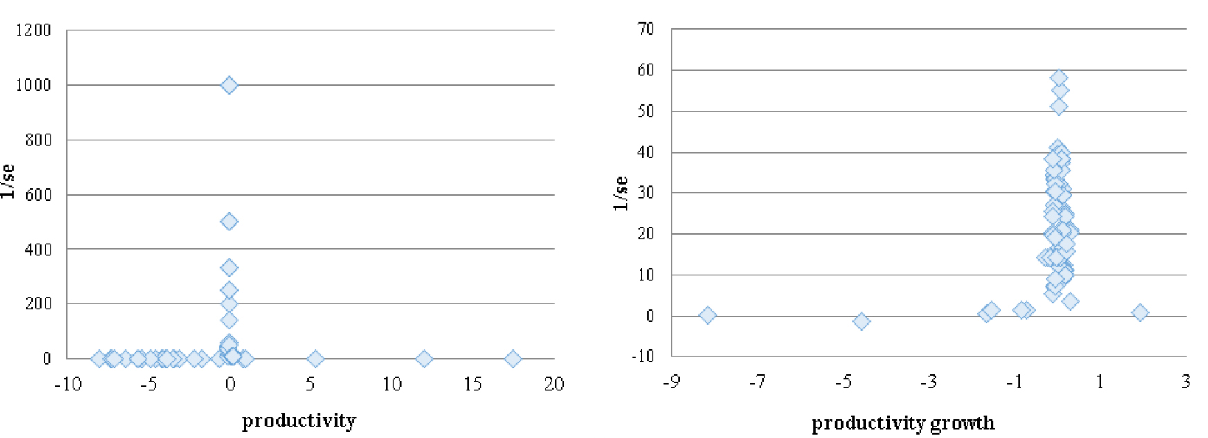
Fig. 1
Funnel plot for productivity and productivity growth. Source: Own study based on literature review.
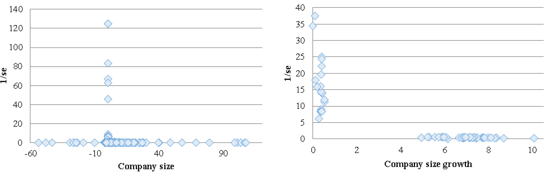
Fig. 2
Funnel chart for the size and growth of the enterprise size. Source: Own study based on literature review
Tab. 2
Test results for the effect of publication selection effect
| Model of variables associated with the impact of subsidies on: | Constant | 1/Sei | ||||
|---|---|---|---|---|---|---|
| Estimate | t | p-value | Estimate | t | p-value | |
| Productivity | −0.53 | −1.86 | 0.067 | −0.00 | −3.56 | 0.001 |
| Productivity growth | 0.15 | 0.27 | 0.791 | 0.02 | 1.06 | 0.294 |
| Company size | 0.86 | 7.91 | 0.000 | 0.13 | 26.03 | 0.000 |
| Company size growth | 3.02 | 10.72 | 0.000 | 0.07 | 2.89 | 0.005 |
[i] Source: Own study based on literature review.
Tab. 3
Patterns
| 2005 | 2006 | 2007 | 2008 | 2009 | 2010 | Number |
|---|---|---|---|---|---|---|
| Sample 4 – the stimulus is a subsidy received in 1 year | ||||||
| 0 | 1 | 0 | x | x | x | 400 |
| x | 0 | 1 | 0 | x | x | 231 |
| x | x | 0 | 1 | 0 | x | 212 |
| x | x | x | 0 | 1 | 0 | 230 |
| Σ1,073 | ||||||
| 0 | 0 | 0 | x | x | x | 250 |
| x | 0 | 0 | 0 | x | x | 113 |
| x | x | 0 | 0 | 0 | x | 150 |
| x | x | x | 0 | 0 | 0 | 137 |
| Σ650 | ||||||
| Sample 5 – the stimulus is a subsidy received in 1 year | ||||||
| 0 | 1 | 0 | x | x | x | 400 |
| x | 0 | 1 | 0 | x | x | 231 |
| x | x | 0 | 1 | 0 | x | 212 |
| Σ843 | ||||||
| 0 | 0 | 0 | x | x | x | 250 |
| x | 0 | 0 | 0 | x | x | 113 |
| x | x | 0 | 0 | 0 | x | 150 |
| Σ513 | ||||||
| Sample 6 – the stimulus is a subsidy received in 2 subsequent years | ||||||
| 0 | 1 | 1 | 0 | x | x | 251 |
| x | 0 | 1 | 1 | 0 | x | 166 |
| x | x | 0 | 1 | 1 | 0 | 134 |
| Σ551 | ||||||
| 0 | 0 | 0 | 0 | x | x | 133 |
| x | 0 | 0 | 0 | 0 | x | 91 |
| x | x | 0 | 0 | 0 | 0 | 90 |
| Σ314 | ||||||
[i] Source: Own study.
[ii] Legend: 1 – means that the company received a subsidy in the given year; 0 – means that the company did not receive a subsidy in that year; x – means that it is not known whether the company received a subsidy or not in a given year.
Tab. 4
Basic descriptive statistics of variables from Sample 4
| Variable | Mean | Standard deviation | First quartile | Median | Third quartile | Minimum | Maximum |
|---|---|---|---|---|---|---|---|
| Added value | |||||||
| 2005 | 76,120.45 | 99,897.67 | 19,569.96 | 37,873.50 | 80,821.06 | 4,420.79 | 404,733.40 |
| 2006 | 83,613.87 | 109,236.30 | 21,594.84 | 42,021.25 | 89,475.37 | 4,834.65 | 441,146.70 |
| 2007 | 94,629.00 | 123,088.10 | 24,375.05 | 49,093.20 | 101,819.00 | 4,881.37 | 496,364.00 |
| 2008 | 11,7970.8 | 175,793.30 | 25,224.33 | 50,964.54 | 112,233.9 | 5,275.76 | 716,159.30 |
| 2009 | 83,833.34 | 106,042.80 | 20,632.80 | 39,637.02 | 90,697.10 | 5,306.50 | 415,198.40 |
| 2010 | 104,954.10 | 142,875.80 | 24,125.26 | 47,695.07 | 110,198.70 | 4,654.68 | 568,563.00 |
| Productivity | |||||||
| 2005 | 1.777 | 1.366 | 0.825 | 1.511 | 2.416 | 0.007 | 11.088 |
| 2006 | 1.673 | 1.247 | 0.803 | 1.471 | 2.195 | 0.001 | 7.840 |
| 2007 | 1.798 | 1.429 | 0.773 | 1.508 | 2.361 | 0.002 | 8.223 |
| 2008 | 1.785 | 1.549 | 0.806 | 1.454 | 2.280 | 0.001 | 12.628 |
| 2009 | 1.767 | 1.635 | 0.755 | 1.391 | 2.357 | 0.001 | 14.452 |
| 2010 | 1.705 | 1.523 | 0.737 | 1.417 | 2.168 | 0.005 | 13.670 |
| Asset growth rate | |||||||
| 2005/06 | 14.562 | 28.806 | 0 | 8.408 | 24.043 | 0 | 241.968 |
| 2006/07 | 15.534 | 37.192 | 0 | 8.647 | 21.646 | 0 | 335.140 |
| 2007/08 | 16.832 | 71.702 | 0 | 5.467 | 18.693 | 0 | 586.462 |
| 2008/09 | 48.259 | 164.670 | 0 | 2.165 | 41.989 | 0 | 496.961 |
| 2009/10 | 86.137 | 199.951 | 0 | 6.950 | 91.379 | 0 | 575.263 |
| ROA (%) | |||||||
| 2005 | 9.212 | 10.042 | 2.393 | 6.129 | 11.957 | 0.070 | 49.916 |
| 2006 | 9.391 | 9.822 | 2.752 | 6.227 | 12.755 | 0.069 | 48.891 |
| 2007 | 9.894 | 10.364 | 2.792 | 6.5807 | 13.163 | 0.052 | 49.187 |
| 2008 | 9.211 | 9.667 | 2.500 | 5.968 | 12.866 | 0.059 | 44.743 |
| 2009 | 9.570 | 10.889 | 2.159 | 6.250 | 12.824 | 0.043 | 48.471 |
| 2010 | 8.547 | 9.460 | 2.313 | 5.574 | 11.256 | 0.047 | 41.475 |
| Size | |||||||
| 2005 | 10.266 | 1.298 | 9.512 | 10.178 | 11.020 | 2.646 | 15.292 |
| 2006 | 10.389 | 1.388 | 9.555 | 10.249 | 11.167 | 5.032 | 15.2177 |
| 2007 | 10.513 | 1.360 | 9.757 | 10.407 | 11.379 | 5.157 | 15.488 |
| 2008 | 10.652 | 1.349 | 9.791 | 10.548 | 11.431 | 5.806 | 14.777 |
| 2009 | 10.525 | 1.316 | 9.705 | 10.376 | 11.250 | 5.315 | 15.471 |
| 2010 | 10.635 | 1.328 | 9.849 | 10.543 | 11.378 | 2.978 | 15.809 |
| Liabilities | |||||||
| 2005 | 0.074 | 0.145 | 0 | 0.005 | 0.081 | 0 | 0.794 |
| 2006 | 0.075 | 0.153 | 0 | 0.004 | 0.071 | 0 | 0.986 |
| 2007 | 0.071 | 0.135 | 0 | 0.010 | 0.087 | 0 | 0.847 |
| 2008 | 0.070 | 0.133 | 0 | 0.005 | 0.082 | 0 | 0.884 |
| 2009 | 0.080 | 0.160 | 0 | 0.007 | 0.083 | 0 | 0.746 |
| 2010 | 0.063 | 0.125 | 0 | 0.003 | 0.070 | 0 | 0.837 |
| Cash flow | |||||||
| 2005 | 0.113 | 0.117 | 0.051 | 0.094 | 0.165 | 0 | 0.686 |
| 2006 | 0.129 | 0.108 | 0.062 | 0.104 | 0.179 | 0 | 0.701 |
| 2007 | 0.112 | 0.112 | 0.050 | 0.096 | 0.160 | 0 | 0.683 |
| 2008 | 0.099 | 0.121 | 0.038 | 0.090 | 0.159 | 0 | 0.810 |
| 2009 | 0.106 | 0.137 | 0.040 | 0.093 | 0.161 | 0 | 0.767 |
| 2010 | 0.099 | 0.125 | 0.043 | 0.091 | 0.143 | 0 | 0.614 |
| Ln(age+1) | |||||||
| 2005 | 2.523 | 0.459 | 2.302 | 2.564 | 2.772 | 1.098 | 3.555 |
| Age | |||||||
| 2005 | 10.765 | 6.368 | 7 | 10 | 13 | 0 | 32 |
[i] Source: Own study based on data from Monitor Polski B.
[ii] Legend: ROA – return on asset.
Tab. 5
Basic statistics of descriptive variables from Sample 4 broken down by subsidised and non-subsidised companies
| Variable | Mean | Standard deviation | First quartile | Median | Third quartile | Minimum | Maximum | |
|---|---|---|---|---|---|---|---|---|
| Added value | ||||||||
| A year before the subsidy | 0 | 79,803.68 | 112,976.00 | 16,537.94 | 36,342.87 | 82,381.98 | 3,284.50 | 455,219.70 |
| 1 | 88,695.01 | 112,648.00 | 21,720.75 | 44,171.46 | 102,177.20 | 3,284.50 | 455,219.70 | |
| A year after the subsidy | 0 | 81,319.56 | 117,916.10 | 16,537.94 | 36,342.87 | 82,381.98 | 3,818.98 | 484,195.40 |
| 1 | 90,074.90 | 117,138.50 | 21,720.75 | 44,171.46 | 102,177.20 | 3,818.98 | 484,195.40 | |
| Productivity | ||||||||
| A year before the subsidy | 0 | 1.7470 | 1.448 | 0.721 | 1.437 | 2.336 | 0.001 | 11.088 |
| 1 | 1.7690 | 1.366 | 0.885 | 1.511 | 2.303 | 0.001 | 12.628 | |
| A year after the subsidy | 0 | 1.690 | 1.425 | 0.645 | 1.428 | 2.315 | 0.003 | 10.323 |
| 1 | 1.779 | 1.757 | 0.823 | 1.412 | 2.250 | 0.001 | 35.423 | |
| ROA (%) | ||||||||
| A year before the subsidy | 0 | 8.604 | 9.760 | 2.032 | 5.232 | 11.987 | 0.003 | 64.416 |
| 1 | 9.489 | 9.908 | 2.840 | 6.539 | 12.609 | 0.001 | 77.003 | |
| A year after the subsidy | 0 | 5.479 | 8.943 | 0.279 | 3.677 | 10.653 | 0 | 26.504 |
| 1 | 5.814 | 9.185 | 0.469 | 4.473 | 10.568 | 0 | 26.504 | |
| Size | ||||||||
| A year before the subsidy | 0 | 10.339 | 1.457 | 9.503 | 10.249 | 11.154 | 2.646 | 15.488 |
| 1 | 10.485 | 1.273 | 9.687 | 10.362 | 11.254 | 6.791 | 15.446 | |
| A year after the subsidy | 0 | 10.474 | 1.479 | 9.602 | 10.351 | 11.325 | 3.247 | 17.646 |
| 1 | 10.608 | 1.282 | 9.807 | 10.506 | 11.355 | 3.336 | 15.446 | |
| Liabilities | ||||||||
| A year before the subsidy | 0 | 0.069 | 0.138 | 0 | 0.004 | 0.071 | 0 | 0.794 |
| 1 | 0.075 | 0.145 | 0 | 0.006 | 0.082 | 0 | 0.794 | |
| A year after the subsidy | 0 | 0.063 | 0.141 | 0 | 0.002 | 0.056 | 0 | 1.309 |
| 1 | 0.083 | 0.155 | 0 | 0.009 | 0.098 | 0 | 1.142 | |
| Cash flow | ||||||||
| A year before the subsidy | 0 | 0.132 | 0.096 | 0.065 | 0.105 | 0.172 | 0.003 | 0.506 |
| 1 | 0.140 | 0.096 | 0.072 | 0.117 | 0.185 | 0.002 | 0.507 | |
| A year after the subsidy | 0 | 0.119 | 0.097 | 0.048 | 0.093 | 0.166 | 0.003 | 0.498 |
| 1 | 0.129 | 0.094 | 0.054 | 0.102 | 0.161 | 0.012 | 0.457 | |
| Ln(age+1) | ||||||||
| A year before the subsidy | 0 | 2.476 | 0.533 | 2.197 | 2.564 | 2.772 | 0 | 3.526 |
| 1 | 2.439 | 0.529 | 2.197 | 2.484 | 2.708 | 0 | 3.555 | |
[i] Source: Own study based on data from Monitor Polski B.
[ii] Legend: ROA – return on asset.
Tab. 6
Results of estimations of logit models – probability of receiving a subsidy
| Variables | Sample 4 (one instalment of the subsidy) | Sample 5 (one instalment of the subsidy) | Sample 6 (two instalments of the subsidy) | |||
|---|---|---|---|---|---|---|
| Parameter | p-value | Parameter | p-value | Parameter | p-value | |
| Added valuet−1 | 0.116 | 0.173 | 0.125 | 0.252 | −0.072 | 0.154 |
| (Added valuet−1)2 | −0.013 | 0.278 | −0.0188 | 0.270 | 0.021 | 0.061 |
| Sizet−1 | 1.263 | 0.000 | 1.315 | 0.001 | 3.908 | 0.000 |
| (Sizet−1)2 | −0.053 | 0.001 | −0.056 | 0.002 | −0.183 | 0.000 |
| Liabilitiest−1 | 0.775 | 0.067 | 0.966 | 0.039 | 1.087 | 0.055 |
| Aget−1 | −0.125 | 0.227 | −0.171 | 0.131 | −0.178 | 0.176 |
| Cash flowt−1 | 0.0108 | 0.049 | 0.016 | 0.010 | 0.049 | 0.109 |
| Sector (base level – industry) | ||||||
| Construction | 0.699 | 0.001 | 0.785 | 0.002 | 0.889 | 0.014 |
| Other | −0.141 | 0.186 | −0.123 | 0.303 | −0.046 | 0.768 |
| Constant | −6.822 | 0.000 | −6.937 | 0.001 | −19.763 | 0.000 |
| Number of observations | 1720 | 1354 | 850 | |||
| Pseudo R2 | 0.023 | 0.027 | 0.035 | |||
| Balancing property | Fulfilled | Fulfilled | Fulfilled | |||
| Test statistics | p-value | Test statistics | p-value | Test statistics | p-value | |
| Linktest | −1.17 | 0.240 | −1.09 | 0.274 | −0.38 | 0.706 |
| Hosmer–Lemeshow test | 13.63 | 0.092 | 10.12 | 0.257 | 6.20 | 0.624 |
[i] Source: Own study based on data from Monitor Polski B.
[ii] Legend: Mcfadden’s Pseudo R2 – balancing property described in the methodology; Linktest – a test checking the correctness of the functional form; the Hosmer–Lemeshow test – a test for the correctness of the functional form of the model.
Tab. 7
Estimation of the mean causal effect treatment on treated units (ATT) for Sample 4
| Variable | ATT | Standard error | Standard error (bootstrap) | Stimulated sample | Control sample | t-test | Better balance? | Are the results stable? |
|---|---|---|---|---|---|---|---|---|
| Nearest-neighbour method (1:1) without replacement | ||||||||
| Productivity a year after the subsidy | 0.069 | 0.077 | 0.071 | 647 | 647 | 0.91 | No | – |
| DProductivityt−1/t+1 | −0.333 | 0.052 | 0.055 | 647 | 647 | −0.64 | – | |
| Asset rate growtht/t+1 | −789,640 | 686,723 | 731,367 | 650 | 650 | −1.15 | – | |
| ROAt+1 | 4,017 | 2,846 | 2,721 | 554 | 554 | 1.41 | – | |
| DROAt−1/t+1 | 1,225 | 2,807 | 2,525 | 554 | 554 | 0.44 | – | |
| Nearest-neighbour method(1:1) with replacement | ||||||||
| Productivity a year after the subsidy | −0.293 | 0.100 | 0.102 | 1066 | 647 | −0.29 | Yes | – |
| DProductivityt−1/t+1 | 0.040 | 0.664 | 0.660 | 1066 | 647 | 0.61 | – | |
| Asset rate growtht/t+1 | −164.064 | 263.881 | 142.815 | 1067 | 650 | −0.33 | – | |
| ROAt+1 | 2.046 | 1.818 | 1.845 | 919 | 554 | 1.13 | – | |
| DROAt−1/t+1 | 2.164 | 1.812 | 1.875 | 919 | 554 | 1.19 | – | |
| Nearest neighbour with calliper(0.25′SD) without replacement | ||||||||
| Productivity a year after the subsidy | 0.059 | 0.082 | 0.816 | 631 | 647 | 0.71 | No | – |
| DProductivityt−1/t+1 | 0.002 | 0.531 | 0.055 | 631 | 647 | 0.04 | – | |
| Asset rate growtht/t+1 | −145.804 | 147.512 | 125.131 | 633 | 650 | −0.99 | – | |
| ROAt+1 | 3.823 | 2.914 | 1.999 | 541 | 554 | 1.31 | No | |
| DROAt−1/t+1 | 2.945 | 2.864 | 2.124 | 541 | 554 | 1.03 | – | |
| Nearest neighbour with calliper(0.1) without replacement | ||||||||
| Productivity a year after the subsidy | 0.112 | 0.079 | 0.084 | 638 | 647 | 1.41 | No | – |
| DProductivityt−1/t+1 | −0.022 | 0.053 | 0.055 | 638 | 647 | −0.42 | – | |
| Asset rate growtht/t+1 | −164.339 | 143.685 | 164.803 | 640 | 650 | −1.14 | No | – |
| ROAt+1 | 4.124 | 2.886 | 2.939 | 546 | 554 | 1.43 | – | |
| DROAt−1/t+1 | 1.314 | 2.846 | 2.643 | 546 | 554 | 0.46 | – | |
| Kernel matching | ||||||||
| Productivity a year after the subsidy | −0.006 | 0.075 | 0.065 | 1066 | 647 | −0.08 | Yes | – |
| DProductivityt−1/t+1 | 0.024 | 0.050 | 0.048 | 1066 | 647 | 0.49 | – | |
| Asset rate growtht/t+1 | −82.209 | 149.109 | 91.829 | 1067 | 650 | −0.55 | – | |
| ROAt+1 | 1.511 | 1.765 | 1.632 | 919 | 554 | 0.86 | – | |
| DROAt−1/t+1 | 1.634 | 1.742 | 1.723 | 919 | 554 | 0.94 | – | |
| Stratification | ||||||||
| Productivity a year after the subsidy | 0.001 | 0.074 | 0.073 | 1070 | 642 | 0.009 | Yes | |
| DProductivityt−1/t+1 | 0.021 | 0.050 | 0.049 | 1070 | 642 | 0.411 | ||
| Asset rate growtht/t+1 | −97.280 | 102.287 | 97.256 | 1070 | 642 | −0.951 | ||
| ROAt+1 | 1.609 | 1.638 | 1.873 | 1070 | 642 | 0.983 | ||
| DROAt−1/t+1 | 1.703 | 1.623 | 1.588 | 1070 | 642 | 1.050 | ||
[i] Source: Own study based on data from Monitor Polski B.
[ii] Legend: ATT – average treatment of treated effect, stimulated sample – the number of units that received a subsidy; control sample – the number of units that did not receive a subsidy; better balance? – ‘yes’ means that after carrying out the t-test for the equality of the mean of individual variables explained in two samples and calculating the standardised bias of variables, it was noticed that the sample balance improved after using data matching, ‘no’ otherwise; are the results stable? – ‘yes’ means that based on the results of the Rosenbaum Bounds test, it was found that the obtained outcomes are free of latent bias, ‘no’ otherwise. ROA – return on asset; SD – standard deviation.
Tab. A1
ATT estimates for Sample 5
| Variable | ATT | Standard error | Standard error (bootstrap) | Stimulated sample | Control sample | Student’s t-test | Better balance? | Are the results stable? |
|---|---|---|---|---|---|---|---|---|
| Nearest-neighbour method (1:1) without replacement | ||||||||
| Productivityt+1 | 0.069 | 0.086 | 0.097 | 512 | 512 | 0.81 | No | – |
| Productivityt+2 | −0.096 | 0.096 | 0.099 | 510 | 510 | −1.00 | – | |
| DProductivityt−1/t+1 | −0.028 | 0.062 | 0.065 | 512 | 512 | −0.46 | – | |
| DProductivityt−1/t+2 | −0.183 | 0.074 | 0.071 | 510 | 510 | −2.46 | No | |
| Asset growth ratet/t+1 | −37.100 | 16.131 | 15.791 | 513 | 513 | −2.30 | No | |
| Asset growth ratet+1/t+2 | 9.971 | 34.773 | 35.496 | 513 | 513 | 0.29 | – | |
| ROAt+1 | 0.888 | 0.998 | 1.125 | 513 | 513 | 0.89 | – | |
| ROAt+2 | 1.156 | 0.711 | 0.810 | 412 | 412 | 1.64 | No | |
| DROAt−1/t+1 | −1.777 | 0.826 | 0.815 | 513 | 513 | −2.15 | No | |
| DROAt−1/t+2 | −2.303 | 0.791 | 0.883 | 412 | 412 | −2.91 | No | |
| Nearest-neighbour method (1:1) with replacement | ||||||||
| Productivityt+1 | 0.039 | 0.109 | 0.098 | 837 | 512 | 0.36 | Yes | – |
| Productivityt+2 | −0.165 | 0.140 | 0.132 | 836 | 510 | −1.18 | – | |
| DProductivityt−1/t+1 | 0.080 | 0.075 | 0.078 | 837 | 512 | 1.06 | – | |
| DProductivityt−1/t+2 | −0.112 | 0.111 | 0.105 | 836 | 510 | −1.00 | – | |
| Asset growth ratet/t+1 | −10.788 | 18.795 | 20.691 | 838 | 513 | −0.57 | – | |
| Asset growth ratet+1/t+2 | 46.294 | 40.202 | 29.200 | 838 | 513 | 1.15 | – | |
| ROAt+1 | 0.866 | 1,242 | 1,051 | 838 | 513 | 0.70 | – | |
| ROAt+2 | −0.268 | 0.829 | 0.678 | 696 | 412 | −0.32 | – | |
| DROAt–1/t+1 | 0,817 | 1,009 | 1,053 | 838 | 513 | 0.81 | – | |
| DROAt−1/t+2 | −0,034 | 0.923 | 0.809 | 696 | 412 | −0.04 | – | |
| Nearest neighbour with calliper (0.25′SD) without replacement | ||||||||
| Productivityt+1 | −0.004 | 0.089 | 0.082 | 498 | 512 | −0.04 | Yes | – |
| Productivityt+2 | −0.157 | 0.102 | 0.102 | 496 | 510 | −1.54 | – | |
| DProductivityt−1/t+1 | −0.015 | 0.063 | 0.064 | 498 | 512 | −0.23 | – | |
| DProductivityt−1/t+2 | −0.161 | 0.080 | 0.084 | 496 | 510 | −2.02 | No | |
| Asset growth ratet/t+1 | −16.426 | 16.711 | 17.092 | 498 | 513 | −0.98 | Yes | – |
| Asset growth ratet+1/t+2 | 4.967 | 33.532 | 35.613 | 498 | 513 | 0.15 | – | |
| ROAt+1 | 0.094 | 1.026 | 1.054 | 498 | 513 | 0.09 | – | |
| ROAt+2 | −0.245 | 0.693 | 0.726 | 400 | 412 | −0.35 | – | |
| DROAt−1/t+1 | −0.476 | 0.811 | 0.780 | 498 | 513 | −0.59 | – | |
| DROAt−1/t+2 | −1.222 | 0.760 | 0.700 | 400 | 412 | −1.61 | No | |
| Nearest neighbour with calliper (0.1) without replacement | ||||||||
| Productivityt+1 | 0.040 | 0.086 | 0.093 | 504 | 512 | 0.47 | No | – |
| Productivityt+2 | −0.156 | 0.095 | 0.102 | 502 | 510 | −1.64 | No | |
| DProductivityt−1/t+1 | −0.043 | 0.062 | 0.056 | 504 | 512 | −0.69 | – | |
| DProductivityt−1/t+2 | −0.232 | 0.075 | 0.076 | 502 | 510 | −3.07 | No | |
| Asset growth ratet/t+1 | −27.875 | 15.225 | 15.800 | 504 | 513 | −1.83 | No | |
| Asset growth ratet+1/t+2 | 38.180 | 35.767 | 37.686 | 504 | 513 | 1.07 | – | |
| ROAt+1 | 0.807 | 1.007 | 1.021 | 504 | 513 | 0.80 | – | |
| ROAt+2 | 1.141 | 0.723 | 0.693 | 405 | 412 | 1.58 | No | |
| DROAt−1/t+1 | −2.055 | 0.829 | 0.957 | 504 | 513 | −2.48 | No | |
| DROAt−1/t+2 | −2.630 | 0.791 | 0.787 | 405 | 412 | −3.32 | No | |
| Kernel matching | ||||||||
| Productivityt+1 | 0.006 | 0.084 | 0.076 | 837 | 512 | 0.07 | Yes | – |
| Productivityt+2 | −0.172 | 0.096 | 0.076 | 836 | 510 | −1.79 | Yes | |
| DProductivityt−1/t+1 | 0.017 | 0.059 | 0.061 | 837 | 512 | 0.28 | – | |
| DProductivityt−1/t+2 | −0.152 | 0.074 | 0.070 | 836 | 510 | −2.05 | Yes | |
| Asset growth ratet/t+1 | −15.013 | 15.632 | 15.744 | 838 | 513 | −0.96 | – | |
| Asset growth ratet+1/t+2 | 35.051 | 31.372 | 27.829 | 838 | 513 | 1.12 | – | |
| ROAt+1 | −0.104 | 0.946 | 0.867 | 838 | 513 | −0.11 | – | |
| ROAt+2 | −0.919 | 0.637 | 0.578 | 696 | 412 | −1.44 | – | |
| DROAt−1/t+1 | −0.209 | 0.760 | 0.733 | 838 | 513 | −0.27 | – | |
| DROAt−1/t+2 | −1.042 | 0.689 | 0.685 | 696 | 412 | −1.51 | – | |
| Stratification | ||||||||
| Productivityt+1 | −0.001 | 0.080 | 0.089 | 831 | 515 | −0.014 | Yes | |
| Productivityt+2 | −0.185 | 0.090 | 0.098 | 831 | 515 | −2.068 | ||
| DProductivityt−1/t+1 | 0.007 | 0.059 | 0.067 | 831 | 515 | 0.112 | ||
| DProductivityt−1/t+2 | −0.172 | 0.069 | 0.066 | 831 | 515 | −2.492 | ||
| Asset growth ratet/t+1 | −17.199 | 15.675 | 14.735 | 831 | 515 | −1.097 | ||
| Asset growth ratet+1/t+2 | 22.340 | 30.035 | 33.496 | 831 | 515 | 0.744 | ||
| ROAt+1 | 2.230 | 2.069 | 1.967 | 831 | 515 | 1.078 | ||
| ROAt+2 | −0.531 | – | 0.679 | 831 | 515 | −0.782 | ||
| DROAt−1/t+1 | 1.608 | 2.040 | 2.033 | 831 | 515 | 0.788 | ||
| DROAt−1/t+2 | −0.980 | – | 0.764 | 831 | 515 | −1.284 | ||
[i] Source: Own study based on data from Monitor Polski B.
[ii] Legend: ATT – average treatment of treated effect; stimulated sample – the number of units that received a subsidy; control sample – the number of units that did not receive a subsidy; better balance? – ‘yes’ means that after carrying out the t-test for the equality of the mean of individual variables explained in two samples and calculating the standardised bias of variables, it was noticed that the sample balance improved after using data matching, ‘no’ otherwise; are the results stable? – ‘yes’ means that based on the results of the Rosenbaum Bounds test, it was found that the obtained outcomes are free of latent bias, ‘no’ otherwise. ROA – return on asset.
Table A2
ATT estimates for Sample 6
| Variable | ATT | Standard error | Standard error (bootstrap) | Stimulated sample | Control sample | Student’s t-test | Better balance? | Are the results stable? |
|---|---|---|---|---|---|---|---|---|
| Nearest-neighbour method (1:1) without replacement | ||||||||
| Productivityt+1 | 0.112 | 0.115 | 0.125 | 302 | 302 | 0.98 | No | – |
| DProductivityt−1/t+1 | −0.112 | 0.090 | 0.084 | 302 | 302 | −1.24 | – | |
| Asset growth ratet/t+1 | −87.850 | 55.623 | 49.382 | 307 | 307 | −1.58 | Yes | |
| ROAt+1 | −14.994 | 18.085 | 20.287 | 307 | 307 | −0.83 | – | |
| DROAt−1/t+1 | −17.203 | 17.715 | 17.676 | 307 | 307 | −0.97 | – | |
| Nearest-neighbour method (1:1) with replacement | ||||||||
| Productivityt+1 | 0.099 | 0.140 | 0.132 | 537 | 302 | 0.71 | Yes | – |
| DProductivityt−1/t+1 | 0.054 | 0.104 | 0.094 | 537 | 302 | 0.52 | – | |
| Asset growth ratet/t+1 | −23.802 | 100.150 | 45.168 | 537 | 307 | −0.24 | – | |
| ROAt+1 | 2.514 | 5.515 | 4.076 | 537 | 307 | 0.46 | – | |
| DROAt−1/t+1 | 2.886 | 5.567 | 3.619 | 537 | 307 | 0.52 | – | |
| Nearest neighbour with calliper (0.25′SD) without replacement | ||||||||
| Productivityt+1 | 0.973 | 0.125 | 0.122 | 286 | 302 | 0.78 | Yes | – |
| DProductivityt−1/t+1 | −0.001 | 0.1026 | 0.114 | 286 | 302 | −0.01 | – | |
| Asset growth ratet/t+1 | −89.562 | 59.594 | 47.787 | 288 | 307 | −1.50 | Yes | |
| ROAt+1 | 1.117 | 3.403 | 3.273 | 288 | 307 | 0.33 | – | |
| DROAt−1/t+1 | 0.775 | 3.474 | 3.030 | 288 | 307 | 0.22 | – | |
| Nearest neighbour with calliper (0.1) without replacement | ||||||||
| Productivityt+1 | 0.118 | 0.118 | 0.123 | 299 | 302 | 1.57 | No | – |
| DProductivityt−1/t+1 | −0.046 | 0.093 | 0.094 | 299 | 302 | −0.49 | – | |
| Asset growth ratet/t+1 | −63.818 | −64.134 | 53.133 | 304 | 307 | −1.00 | – | |
| ROAt+1 | 2.096 | 3.238 | 3.386 | 304 | 307 | 0.65 | – | |
| DROAt−1/t+1 | −0.448 | 3.304 | 3.275 | 304 | 307 | −0.14 | – | |
| Kernel matching | ||||||||
| Productivityt+1 | 0.044 | 0.109 | 0.102 | 537 | 302 | 0.40 | Yes | – |
| DProductivityt−1/t+1 | −0.196 | 0.084 | 0.092 | 537 | 302 | −0.23 | – | |
| Asset growth ratet/t+1 | −19.336 | 62.620 | 33.639 | 537 | 302 | −0.31 | – | |
| ROAt+1 | 2.411 | 3.374 | 4.133 | 537 | 307 | 0.71 | – | |
| DROAt−1/t+1 | 2.533 | 3.430 | 3.428 | 537 | 307 | 0.74 | – | |
| Stratification | ||||||||
| Productivityt+1 | 0.093 | 0.113 | 0.113 | 542 | 302 | 0.819 | Yes | |
| DProductivityt−1/t+1 | −0.027 | 0.094 | 0.093 | 542 | 302 | −0.288 | ||
| Asset growth ratet/t+1 | −21.846 | 31.758 | 35.329 | 542 | 302 | −0.688 | ||
| ROAt+1 | 1.945 | 3.393 | 3.231 | 542 | 302 | 0.573 | ||
| DROAt−1/t+1 | 2.196 | 3.446 | 3.437 | 542 | 302 | 0.637 | ||
[i] Source: Own study based on data from Monitor Polski B. Legend: ATT – average treatment of treated effect; stimulated sample - the number of units that received a subsidy; control sample – the number of units that did not receive a subsidy; better balance? – ‘yes’ means that after carrying out the t-test for the equality of the mean of individual variables explained in two samples and calculating the standardised bias of variables, it was noticed that the sample balance improved after using data matching, ‘no’ otherwise; are the results stable? – ‘yes’ means that based on the results of the Rosenbaum Bounds test, it was found that the obtained outcomes are free of latent bias, ‘no’ otherwise. ROA – return on asset.