

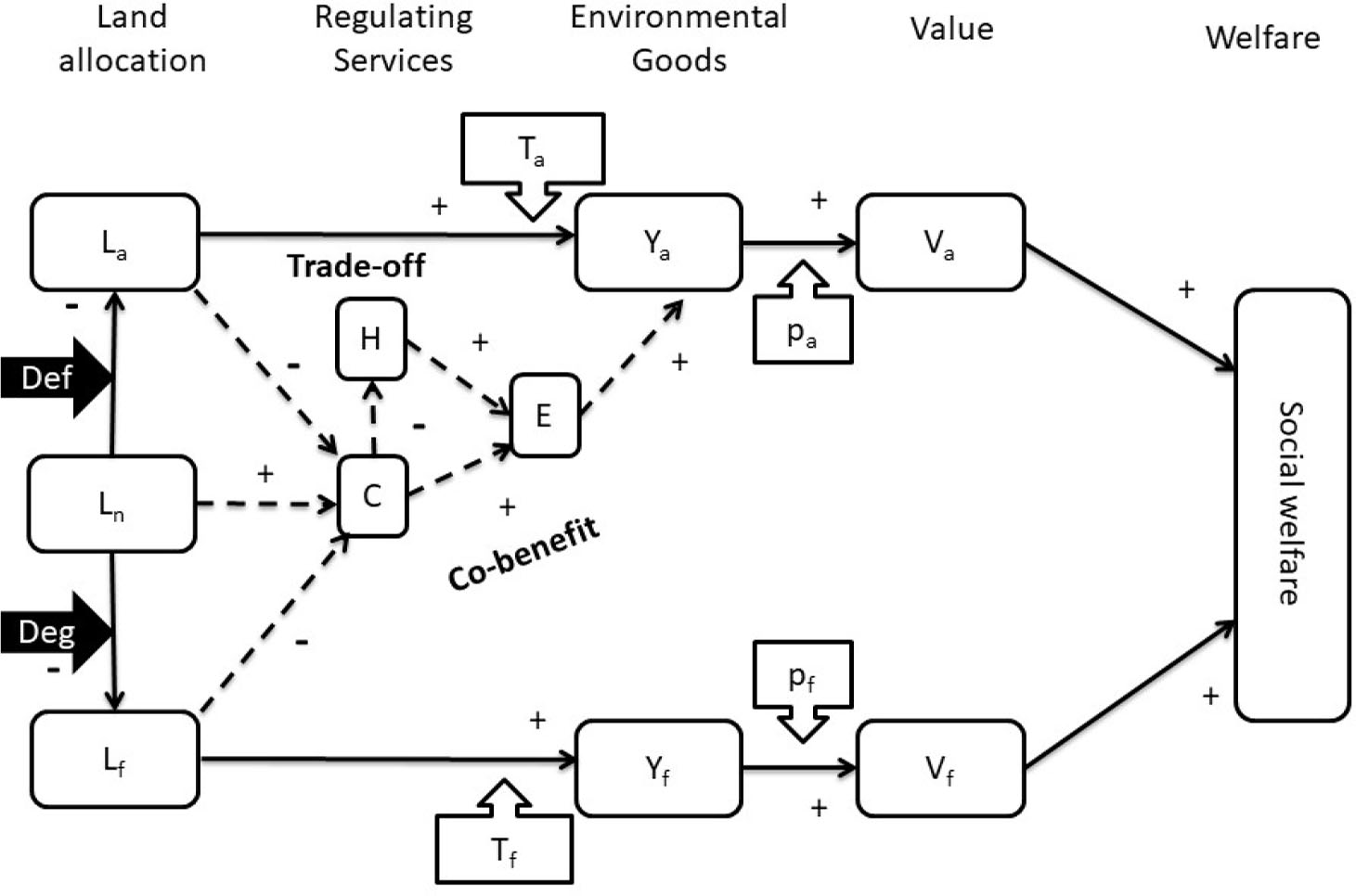
Fig. 1
Conceptual map for tropical deforestation and forest degradation.
Source: author's own elaboration.
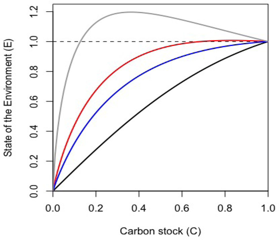
Fig. 2
Effect of land use change on the overall provision of regulating ES given different parameters specification.
Source: author’s own elaboration. Notice that equation 5 is defined in terms of C and H, however, H is a function of C. Thus, the resulting curve can be plotted using only in terms of C. Parameter specification is as follows:
Black curve: s = 0.7, α = 0.5
Blue curve: s = 0.4, α = 0.7
Red curve: s = 0.5, α = 0.7
Gray curve: s = 0.25, α = 0.75
Tab. 1
Parameters of the model.
| Fixed parameters | |||
|---|---|---|---|
| Parameter | Value | Description | Source |
| α | 0.3 | Exponent agriculture land in production function | Jointly determined to replicate late transition phase as reported in Hosonuma et al. 2012 |
| β | 0.7 | Exponent agriculture land in production function | |
| pa | 1.3 | Output price agriculture | |
| pf | 1 | Output price forestry | |
| γ | 0.25 | Exponent of state the state of the environment in externality function | Value selected to replicate forest cover along the different phases of forest transition as reported in Hosonuma et al. 2012 |
| Cmax | 1 | Maximum carbon stock (Normalized) | The values could not be derived from the literature directly. Nevertheless they are consistent with what can be found there |
| 1 | Land endowment (Normalized) | ||
| 1 | Labor endowment (Normalized) | ||
| k | 0.25 | Inflection point of Hill function | Assumption consistent with mathematical formulation |
| n | 1 | Steepness Hill functions | Assumption consistent with mathematical formulation |
| Random Parameters | |||
| s | N(0.5, 0.083) | Carbon share | Assumption consistent with mathematical formulation* |
| α | U(0.1 – 0.85) | Elasticity of substitution | Assumption consistent with mathematical formulation |
| d | U(0.1 – 0.5) | Degradation | Specht et al 2015 and Gerwing 2002 |
Tab. 2
Policy configurations.
| Policy/configuration | Ln quota* (%) | Compensation+ | Agr | For |
|---|---|---|---|---|
| Unregulated | 0 | No | - | - |
| Reserve | 7 | No | - | - |
| Compensation | 7 | Yes | - | - |
| Mitigation | 7 | No | Tax on C | - |
| Adaptation | 7 | No | - | Subcidy on H |
| Policy integration | 7 | No | Tax on C | Subcidy on H |
Source: Author’s own elaboration.
Notes:
+ When compensation mechanism is active (yes), the amount of land kept as natural forest (Ln) is compensated based on its opportunity cost (r), otherwise compensation is zero, see equation (2) and appendix A.1 for details.
A tax implies that t > 0, while a subsidy means that t < 0. Otherwise, t = 0. See equation (1) and appendix A.2. for details.
Tab. 3
Variables calculated for the numerical solution of the model and their use.
| Economic subsectors | ||
|---|---|---|
| Variable | Description | Use |
| Πj | Profit | Not reported but known to be zero |
| Yj | Production | Calculate GDP |
| Lj | Land use | Model calibration |
| Tj | Labor use | Not reported |
| λj | Shadow price | Not reported |
| Factors Markets | ||
| w | Wage rate | Not reported |
| r | Opportunity cost of land | Calculate GDP (depending on policy configuration) |
| Ecologic sector | ||
| C | Carbon stock | Mitigation indicator |
| H | Hydrological services | Indirectly contained in GDP calculation |
| E | State of the environment | Calculate GDP |
[i] Source: author’s own elaboration.
Tab. 4
Average forest cover in 2010 per phase of forest transition process.
| Phase | Number of countries | Average forest cover (%) |
|---|---|---|
| Pre transition | 13 | 69.9 |
| Early transition | 39 | 46.6 |
| Late transition | 33 | 21.3 |
| Post transition | 15 | 27.3 |
[i] Source: author’s own elaboration based on World Bank data.
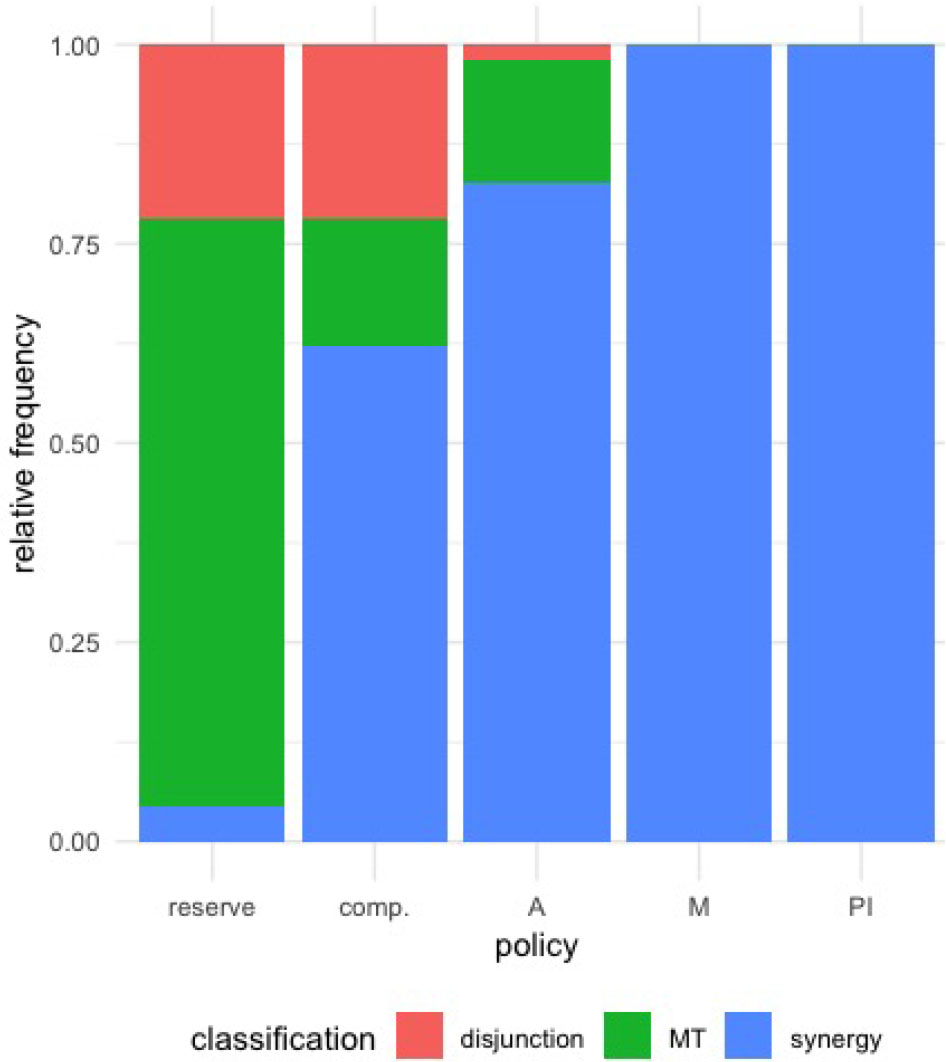
Fig. 3
Classification frequency of different policy scenarios.
Source: author's own elaboration.
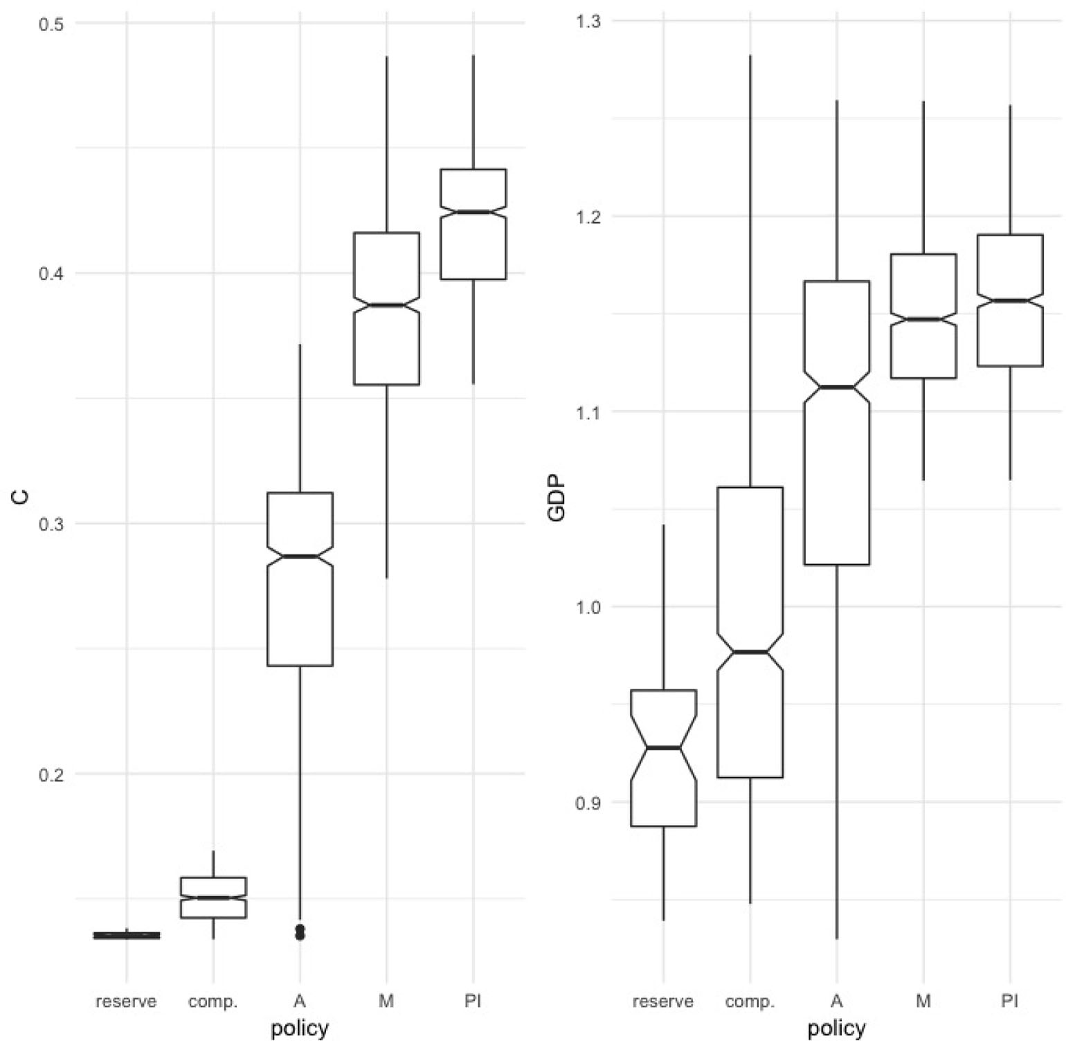
Fig. 4
Environmental (C) and welfare indicators (GDP) of synergic outcomes by policy
Source: author's own elaboration.
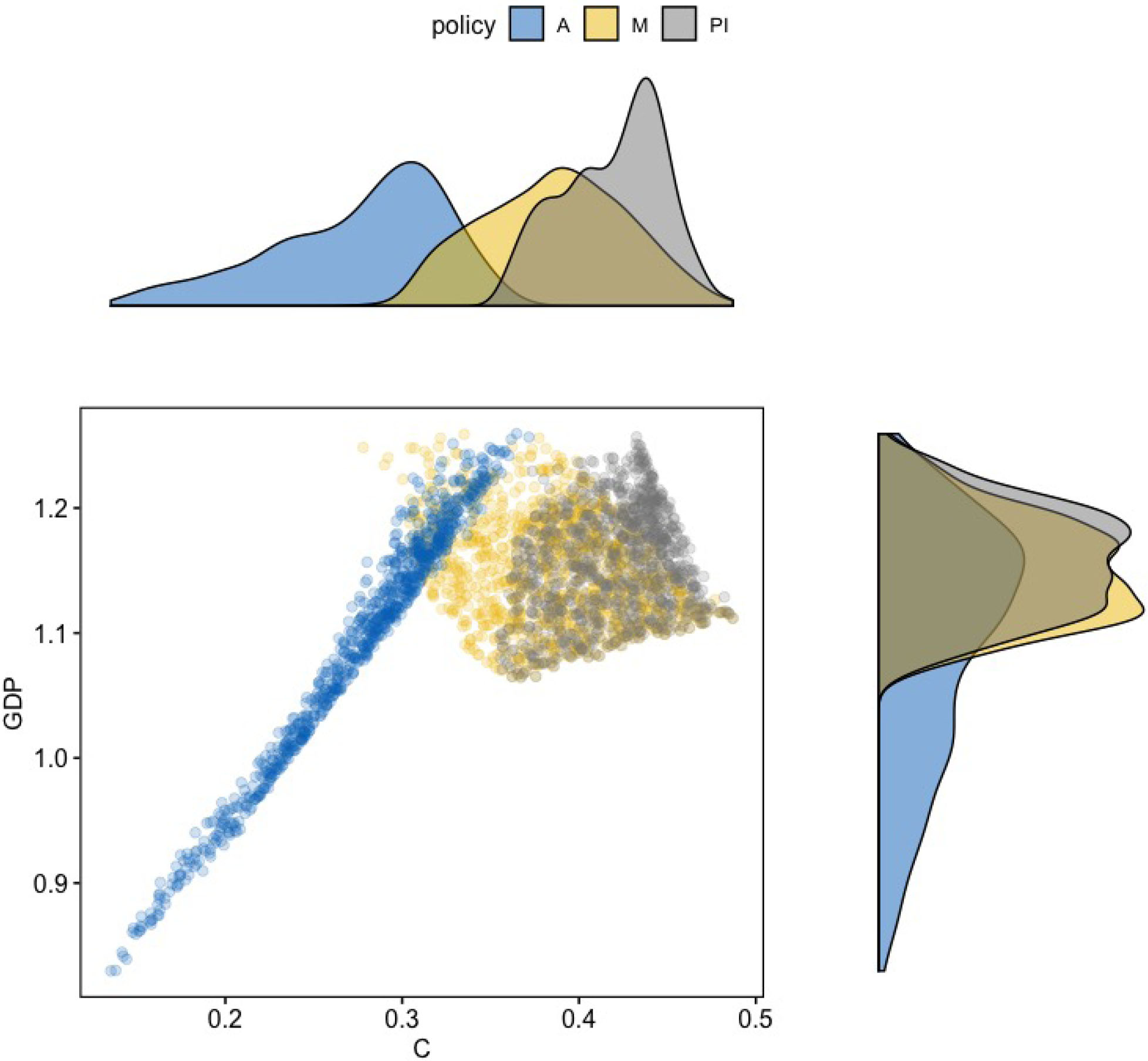
Fig. 5
Environmental and welfare indicators of alternative policy scenarios.
Source: author's own elaboration.